Using year as covariate for anual density estimations

[Pamela Narváez]

Hello, 

I apologize if something like this has been asked before.

We’re working on calculating the densities of a few lemur species over a 5 year period (2015-2019). We are interested on how the densities of these species have changed with changes in forest fragment size, and ideally, we would like to estimate the density of each species per year.  We have 37 line transects (length 500m), and we walked them between 6 and 30 times every year.  

Towards the last 2 years of the 5-year period, we have been getting fewer and fewer observations (e.g., from 53 in 2015 to 12 in 2019 for one species), so we’re having troubles with some of the results. From what I read in someone else’s email chain, Dr. Buckland mentioned that it’s ok not to have >60 or even >80 sightings in line-transect surveys if you get good fits and the detection function makes sense. However, the observations we have might be a bit too low to continue the analysis (I tried it and it doesn’t look great). 

I’ve already tried covariate modeling with rare species following your example (http://examples.distancesampling.org/Distance-spec-covar/species-covariate-distill.html ). However, the density estimates for the more common species appear considerably smaller than what I would get if I run the analysis of those species individually.  

I was thinking about combining the 2015-2019 data for each individual species and then using year as a covariate. Do you think this would be a good approach?

Thank you so much for your time!!

Pamela Narváez-Torres
University of Calgary

[Eric Rexstad]

Pamela

Your suggestion about combining data across years (rather than across species) follows the same principle.  Combining years assumes the detection functions for all years share the same key function, but the scale parameter of the key function differs between years.  It seems plausible that detectability for a species shares a key function across years but that inter-annual differences may cause the scale parameter to differ between years.

--
You received this message because you are subscribed to the Google Groups "distance-sampling" group.
To unsubscribe from this group and stop receiving emails from it, send an email to distance-sampl...@googlegroups.com.
To view this discussion on the web visit https://groups.google.com/d/msgid/distance-sampling/db391aeb-0709-44bb-b5c7-35314a4abb71n%40googlegroups.com.

-- 
Eric Rexstad
Centre for Ecological and Environmental Modelling
University of St Andrews
St Andrews is a charity registered in Scotland SC013532

[Pamela Narváez]

Dear Eric, thank you so much for the reply! I tried doing it for one species,  but the densities keep coming up as zero. Here’s the data and code I am using. Any comments would be really helpful!

lem_year<- read.csv(file="Lemur_covyear.csv", sep=",",h=T)

lem_year$year<-as.factor(lem_year$year)

DS_lemY<- ds(data = lem_year,

                key="hn",

                formula=~year)

 summary(DS_lemY)

gof_ds(DS_lemY)

plot.with.covariates(DS_lemY)

ds_cov_lemY <- dht2(ddf=DS_lemY, flatfile=lem_year,

                  strat_formula = ~year, 

                  stratification = "object")

 

Thanks again!

 

Pamela

[Eric Rexstad]

Pamela

The solution is actually more simple than your approach.  For the data you provides, we can treat year as a stratification factor.  This simple solution won't work if you have geographical strata as well as yearly surveys.  I simply copy your `year` covariate into the `Region.Label` field.  This way, there is no need to invoke `dht2`.

I've also fooled around a bit assessing whether detectability actually changes by year. I've also introduced a units conversion so that density is reported in lemurs per sq km.

library(Distance)

lem_year<- read.csv(file="C:/Users/erexs/Documents/My Distance Projects/Pamela/Lemur_covyear.csv")

conversion <- convert_units("meter", "meter", "square kilometer")
lem_year$Region.Label <- lem_year$year
DS_lemR<- ds(data = lem_year,
             key="hn",
             formula=~Region.Label,
             convert.units = conversion)
summary(DS_lemR)
gof_ds(DS_lemR)

If you examine the summary() output, you will see year-specific estimates are provided:

Density:
  Label  Estimate        se        cv      lcl       ucl        df
1  2014 10.846999 3.2701748 0.3014820 5.999292 19.611876  50.60852
2  2015  7.193801 2.1466990 0.2984096 3.991637 12.964797  42.98662
3  2016  4.180019 1.2379703 0.2961638 2.336603  7.477762  52.88349
4  2017  4.138706 1.7936978 0.4333959 1.798687  9.522993  49.98898
5  2018  2.755814 1.2932233 0.4692709 1.138530  6.670455 111.57897
6  2019  3.922302 1.8101181 0.4614938 1.623101  9.478433  50.53604
7 Total  5.351963 0.8017811 0.1498107 3.990059  7.178718 213.88215

But the summary also shows the beta parameters associated with the year-specific estimates of the shape parameter of the half-normal key function:

Detection function parameters
Scale coefficient(s):  
                     estimate        se
(Intercept)       2.111800931 0.1330146
Region.Label2015  0.004741692 0.1680775
Region.Label2016  0.327478413 0.2087262
Region.Label2017  0.216059594 0.2441551
Region.Label2018  0.086051672 0.3725973
Region.Label2019 -0.361882282 0.2386520

The standard errors of these betas are of the same size or larger than the estimates themselves.  This suggests there is not a strong "year" signal in the shape of the detection functions.  Perhaps a model with a pooled detection function would be equally suitable for these data:

DS_lemCons<- ds(data = lem_year, key="hn", convert.units = conversion)
AIC(DS_lemR, DS_lemCons)
summary(DS_lemCons)

> AIC(DS_lemR, DS_lemCons)
           df      AIC
DS_lemR     6 960.9689
DS_lemCons  1 959.9827

The AIC comparison implies there is little difference between the models, both of which fit the data.

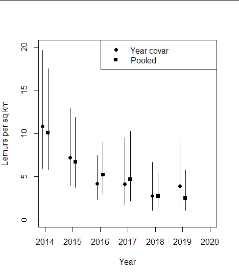
Having a look at the point and interval estimates of the two models bears out the minute difference between the models.

# plotting
dens_yrcov <- DS_lemR$dht$individuals$D
dens_yrcov$year <- as.numeric(dens_yrcov$Label) - 0.1
plot(dens_yrcov$year, dens_yrcov$Estimate, ylim=c(0,20), xlim=c(2014,2020), pch=19,
     xlab="Year", ylab="Lemurs per sq km")
segments(dens_yrcov$year, dens_yrcov$lcl, dens_yrcov$year, dens_yrcov$ucl)


dens_cons <- DS_lemCons$dht$individuals$D
dens_cons$year <- as.numeric(dens_cons$Label) + 0.1
points(dens_cons$year, dens_cons$Estimate, ylim=c(0,20), pch=15)
segments(dens_cons$year, dens_cons$lcl, dens_cons$year, dens_cons$ucl)
legend("topright", pch=c(19,15), legend=c("Year covar", "Pooled"))

To view this discussion on the web visit https://groups.google.com/d/msgid/distance-sampling/78b3c21f-f750-4d57-9849-dc73f1839472n%40googlegroups.com.

[Pamela Narváez]

Thank you very much Eric! I really appreciate the help! I’ll try this out with some other lemur species :)

Pamela 

_____________________

Pamela Narvaez-Torres

University of Calgary

<fdjeehndecciinfo.png>

[Hannah Madden]

Good morning,

I read with interest this approach for analyzing data on a declining species. We have the same issue with a bird species (I have collected survey data between 2016 and 2021). I was trying to run the same analysis but keep getting an error: 

Error in checkdata(data, region.table, sample.table, obs.table, formula) : 

  A sample has a non-unique "Effort", check data!

It's probably simple but I cannot figure out how to fix the issue..... 

Hannah

[Eric Rexstad]

Hannah

Sorry, I can't diagnose your problem from the information you've provided.  Are you willing to send along the data file (off the list) and I can have a look.

To view this discussion on the web visit https://groups.google.com/d/msgid/distance-sampling/dd916cb4-df10-461d-b4af-58415c1616fan%40googlegroups.com.

[Hannah Madden]

Hopefully I sent it to your correct email address - thank you!

[Pamela Narváez]

Hello again,

I’ve emailed before to ask for help on calculating densities for a few lemur species over a 5 year period. Dr. Rexstad suggested treating year as a stratification factor or using a model with a pooled detection function and these suggestions worked great! Following his suggestion, I calculated densities for 4 species and got estimations per year (2015-2019). 

However, now that we’re looking into what kind of models we can run (most likely linear models), we’re running into issues due to our low number of observations (1 density estimation per year for 5 years).  We’re interested in the effect that forest loss (and other disturbance-related variables) has on the density of these lemur species over a 5-year period. We’re working with satellite imagery to estimate forest loss per year, so, for each year and for each species we will get a value for forest loss and a density estimation (5 values). As you can imagine, modelling this with only 5 values in our dependent variable is really tricky. 

I was going over the Distance Sampling: Methods and Applications book (Buckland et al., 2015), especially over Ch. 8, and was thinking about the possibility of using count models (e.g., Poisson) + covariates (e.g., forest loss) instead of using a separate linear model. Do you think this would be a possibility that would help me answer my research question? I might be overcomplicating things so any suggestions will be highly appreciated!

Thank you so much!

Pamela Narváez

PhD student

University of Calgary

Just as a reminder, we conducted repeated surveys over a 5 year period on 35 line transects (length 500m) in Madagascar. The transects are in 5 forest fragments, and the te transects have been walked at least 10 times per year. 

[Eric Rexstad]

Pamela

The methods described in Sections 8.5.1 and 8.5.2 of Buckland et al. (2015) are data-hungry.  Note the number of sites in those studies are 446, compared to the 35 you have.  I suspect your habitat measure of interest (forest cover) does not measurably change between the multiple walks per year; and as I recall you are unlikely to produce defensible density estimates on a per-visit basis.  This leads me to suspect it might still be difficult to assess the effect of habitat on animal density.

Nevertheless, the attached document (for an upcoming introductory workshop) might be adaptable to your situation.  Before going down this route, you should do lots of exploratory work to assess whether there might be a signal about forest cover in your data.  The code has not been generalised hence is likely to require work to conform to your situation.

To view this discussion on the web visit https://groups.google.com/d/msgid/distance-sampling/87335ca1-988c-4fce-8dd6-af83ed933264n%40googlegroups.com.

[Pamela Narváez]

Dear Dr. Rexstad,

Thank you so much for the information. I’ll work on what you suggested! 

Although we’re still working on getting yearly forest size, some preliminary analysis show a significant effect of forest size on encounter rates; and contrary to what one would expect, we are looking at a clear decrease in forest seize and decrease in density in 4 species.

Thank you so much!

Pamela 

<countmodel.html>

[Jonathan Felis]

Hello,

I have a question related to this thread, and have also seen references in other threads to my question but still am a little bit unsure of how to proceed. Any feedback would be very appreciated. I inherited a multi-year dataset of vessel-based line-transect survey data for a rare seabird species. The study area is divided into two strata of equal area, wherein Region 1 has much higher birds densities and also receives 3x as much linear effort per survey compared with Region 2. Each stratum is surveyed 5-10x annually (always the same # surveys per stratum in any given year, transect lines are random within strata). Historically, detection functions have been modelled annually to produce annual abundance estimates for the entire study area, however total annual detections are typically 50-150 sightings. Annual detection models can be reasonable, however in some cases the detections are few and in general the sample sizes make it difficult to include what might be important covariates in annual models (a two-level categorical ocean conditions variable, and a two-level cluster size [1 or 2] variable). Finally, I should emphasize that encounter rates in Region 2 are typically very low or zero. I've considered dropping it from analysis, but would like to maintain for now if possible. 

In general, I'd like to create a multi-year detection model (and evaluate covariates) that I can then apply annually for annual abundance estimates. From what I've read on several posts here, two-level stratification (for example, Year+Region) is tricky or not really tested yet with dht2(). I've started thinking that perhaps I could do something like:

let "mydata" = flatfile of combined observations, effort, area, year (Year1, Year2), region (Region1, Region2)

ddf_pooled <- ds(data=mydata, key="hr", formula=~ClusterSize, ...)

Year1result <- dht2(ddf=ddf_pooled, flatfile=filter(mydata, year==Year1), strat_formula=~region, stratification="geographical")

Year2result <- dht2(ddf=ddf_pooled, flatfile=filter(mydata, year==Year2), strat_formula=~region, stratification="geographical")

Does this approach conceptually work? If so, next question relates to cluster size for density/abundance estimates. Even in the simpler case of a single year detection model and study area abundance estimate incorporating both strata, from what I can tell mean cluster size and variance are being calculated at the stratum-level. In our case, there is no information suggesting cluster size varies by stratum, and perhaps more importantly the low numbers of detections in Region2 make this approach a bit silly. For example, for ten surveys in Region2 in a given year, the number of detections per survey is often something like c(0, 1, 0, 0, 0, 2, 0, 0, 0, 0). For annual estimates, and/or for the multi-year approach I tried to outline above, is there a way to force cluster size to be estimated across strata?

As I mentioned earlier, I am also considering dropping Region2 entirely from analysis. In that case, I could follow other examples shown on the forum to create a pooled multi-year detection model and set Region.Label=Year in ds(). 

Thanks for any thoughts or suggestions.

-Jon

[Eric Rexstad]

Jonathan

I'm not sure I can come to grips with all the details of your design and intended estimates, but I'll offer a couple of comments.

Your are correct that two-level stratification is not yet possible with the Distance package.  Instead of treating year as a stratum, simply include year as a covariate in the detection function along with other covariates such as region and group size; then employ the strategy you described in your code.

As for using study area-wide estimates of groups size, afraid that cannot be carried out with the Distance package.  You could perform the calculation manually using the estimate of mean group size (and standard error) for the entire study area, and combine with stratum-specific estimates of group abundance.  However, I would be cautious of this approach.  You note there is little evidence of stratum-specific differences in group size, but you note that the data you have from Region 2 is sparse--suggesting you have a poor idea of what Region 2 group size might be.  I don't see harm in using region-specific estimates of group size; it reflects the information you have.

In general it does sound like Region 2 is going to be your burden to bear.  Given the survey design with 1/3 the effort allocated to Region 2, you will struggle for detections.

To view this discussion on the web visit https://groups.google.com/d/msgid/distance-sampling/aa41a04e-8d0e-4256-bb66-a4ba44fdd97cn%40googlegroups.com.

[Jonathan Felis]

Thank you for getting back to me with the helpful thoughts. I apologize if my description of the original study design was a bit convoluted, I'm still coming to grips with some aspects of it myself as I explore the data more fully! I'd be very happy to share the data with you directly if you don't mind taking a look, and/or an RMarkdown output with some of what I've explored so far. And I'd be happy to talk off-list if that's better, I'd appreciate the help!

Perhaps it's worth backing up a bit. And also let's ignore the two regions for now and just focus on the original Region 1 (where most detections occur). The original motivation for this study was to estimate annual population size and monitor for changes in annual estimates over time (now a 20-year time series). Based on logistical and funding constraints, typically 5-10 line transect surveys were conducted annually, each one a randomized zig-zag transect of similar length through the study area. Detections per year were ~40-400. Historically, detection functions and abundance estimates have been produced annually using only that year's data. Also, in some years exact distances were used in modeling, while in other years distances were grouped (but not always the same way). In some years covariates (like sea state) were evaluated and in other years they were not. As I inspect the data myself and consider working with a single model with "Year" as a covariate (as well as perhaps a few others like sea state), I think I'm getting hung up on what might be the best path forward given some inconsistencies in data across years. In an ideal world, it seems most efficient to work with a single, global model across years (with year as covariate), and to hold constant decisions such as distance grouping (both it's use and the specific cut points) and covariate inclusion (e.g. sea state). 

However, I note these issues with initial data inspection:

1. Perpendicular distances (95% are <=120m from the line) were calculated from radial distance and angle estimates. While there are some obvious heaping issues for original radial distances and angles (by fives), calculation of perpendicular distance smears most of that out, except for some obvious heaping of perpendicular distance at 0 due to angles being too often rounded to zero. This spike in the detection distance histogram near zero is apparent in some, but not all, years. Note that most years of historical analysis used cut points = c(0, 20, 40, 60, 80, 100, 120), which I think helped accommodate this. 

2. For a specific 3-year period (corresponding to a specific survey crew), there is evidence from the detection distances that observers were not adequately guarding the line. The number of detections initially increases from 0 out to ~30m from the line, then starts decreasing beyond.  This may be in tandem with birds slowly swimming away from the boat before detection. In a easy world, I could assume that the line wasn't adequately guarded but that birds close to the line were all ultimately detected, just a little further away from the line (up to 30m?) than where they would have been detected if the line had been adequately guarded. Note that in these years, historical analysis used cut points = c(0, 30, 60, 70, 80, 90, 100, 110, 120), presumably to accommodate this issue and create a better shoulder for the model. 

When confronting these sorts of issues across a multi-year data set, is there a best approach to building a global model of all years combined? Or is it best to not do so? A few options I've played with:

1. A single model with Year (levels=20) as covariate, as well as Sea State (levels=2) and Cluster Size (levels=2). Distances are grouped. Not enough DOF for GOF test. I set formula=~Year and Region.Label=Year in call to ds() to get annual estimates as output.

2. A unique model for each Year, also evaluating Sea State and Cluster Size covariates. Also allowing for different key functions for each Year potentially. Distances are either grouped the same in each Year (and same as (1) above) to allow AIC comparison between individual and global model, or not grouped the same in order to better accommodate Year-specific data collection issues. GOF tests possible.

3. Also note that there have been some significant survey crew and platform (vessel) changes over the years. I've considered lumping years into a few specific "Eras" (levels=5) corresponding to when crew and/or survey platform were held constant, as I'd expect the data within each "Era" covariate level to be similar across years included with regards to detection. If I replaced "Year" with "Era" in (1) and (2) above, this would also increase the number of detections for the covariate levels in the global model as well as the unique models (remembering that annual detections are sometimes only ~40, below recommended). Set formula=~Era and Region.Label=Year in call to ds() to get annual estimates as output. 

To circle back around, the goals are to estimate annual abundance and hopefully detect changes therein in a cohesive way, but we'd also like to ask other questions of this dataset. For example, we're interested in temporal post-stratification: are density estimates similar or different early- versus late-season? How about CVs? As there are not enough surveys (samples) to answer this question annually, I assume with a global model we could set Region.Label=Season in the call to ds()? Also we'd like to dovetail this detection model into dsm() for some further work. It seems most efficient to have some sort of global model for all years of data to move forward, if possible. 

Thank you again for your time!

-Jon

[Eric Rexstad]

Jonathan

Thanks for your follow-up.  You are asking the right questions.  For many of your questions, there isn't a "cookbook" answer that says "do this".

The funding constraints resulting in the survey design that you inherited hasn't done you many favours.  In the face of sparse data, decisions associated with analysis can have more profound consequences than when a study has a richer pool of data.

I'm comfortable with your suggestion of ignoring the second stratum that is more data poor than the first stratum; that simplifies things a bit.  I might also suggest doing the same with sea state, relying upon the pooling robustness property of distance sampling to produce unbiased estimates even when ignoring some factors that might affect detectability.

I don't know what your exploratory analysis might suggest about the effect of group size.  Do your organisms congregate in groups of size 1-10 or groups of size 1-10000?  If the former, the effect of group size might be small or you could consider treating detection of a group of size 5 as 5 detections of singles all at the same perpendicular distance--thereby diminishing the group size issue.

That might prune off a few issues to make your work more tractable.

Regarding your interest in squeezing further information from the data set, that is an understandable desire, but you've not said anything about the design of the survey to allocate effort among seasons, so you'd need to do exploratory work to see how surveys are temporally distributed within seasons and whether this might be confounded with other factors (crew A surveyed early in the season, while crew B surveyed late in the season; or through time, surveys tended to be conducted earlier (or later) in the season).  Given your concern that data are already spread a bit thin, I'm dubious of the chances of a clear picture about seasonal effects upon abundance; but then I'm a pessimist.

For your remaining questions, dealing with fitting detection functions with possible evasive movement and varying amounts of heaping, the only general statements I can make are that you are trying to estimate the shape of the detection *process*, with vagaries of data quality hindering that intention.  Beyond that, we'd probably be best to go off-list and report any revelations back to the list.

To view this discussion on the web visit https://groups.google.com/d/msgid/distance-sampling/a8681eb5-a694-41d5-bc7d-356f1dfc1954n%40googlegroups.com.