Doubts with ctmm.fit, akde calculation and PMF/PDF

[Elena Bravo]

Hi Chris, 

I wanted to ask you a few questions. 

The first one is regarding what is better to use ctmm.fit or ctmm.select, as I understand ctmm.select is more exact but also it takes more time. The thing is that I have large data sets of even 60 thousand locations and a few individuals. Therefore calculating ctmm.select and the akde takes a lot of time. So I wonder if I could use instead ctmm.fit? what would you do?

The second question is regarding the time the akde takes to calculate. For some individuals is okey but for others it never ends, and it doesnt matter if the dataset has 60 or 1 thousand location. Adding the following code I could calculate the akde faster: 

fast=FALSE,PC='direct'

I did it for a dataset of 1600 data poits, could that be to much? The problem is that I have even larger datasets with the same problem. I have tried also to put trace=TRUE and the bandwith size that I usually get is: 

Default grid size of 8.85 minutes chosen for bandwidth(...,fast=TRUE).

I also tried using a smaller dt, like dt=1, but it didn't seem to make much difference. 

If you want to check the data sets (i upload two, one with a lot of locations and one with almost 2000) and the code Im using is in the following carpet:

https://drive.google.com/drive/folders/18vOCGfUtQzvH-CbXu4ianQndC9aVr7Zi?usp=sharing

Finally the last question, regards the use of PDF or PMF. Im not sure wich want to use to compare the probability of presence with the location of other infraestructure such as wind turbines. 

That would be all, thanks in advanced!

[Christen Fleming]

Hi Elena,

If all of your data are well sampled, of the same species, and ctmm.select() always comes out as OUF anisotropic, then it can be okay to only use ctmm.fit() for speed. You can also consider parallelizing your loop over individuals, or both.

With weights=TRUE, you really only need this for irregularly sampled data and I have pushed some updates to Github that try to choose a faster default grid size that still works. Please try that and see if the default comes out larger and it runs faster.

fast=FALSE,PC='direct' will likely be a fast option for 1,600 data points and doesn't require a choice of dt, but this will slowdown considerably with 60,000 data points (by a factor of 50k), where as the fast algorithm will only slow down slightly (by a factor of 30).

PMF is scale dependent and is for doing calculations, like numerical integration for expectation values. If you want to do comparisons across individuals, then you likely want the PDF.

Best,

Chris

[Elena Bravo]

Hi Chris!, 

Thanks! You helped me a lot. Just one thing, I forgot to add that with the akde I was already using weights=TRUE, this would be my line of code: 

  UDw <- akde(Nombre_individuo_tel,model,weights=TRUE,trace=TRUE,grid=list(dr=100,align.to.origin=TRUE))

I've tried calculating it both with the version 0.6.1. and 0.6.2. What else can I try?

Thanks again :)

[Christen Fleming]

Hi Elena,

If weights=TRUE is extremely slow with the default settings on a very recent development version of the package (within the last couple of weeks), then if you can send me a minimal working example (data + script), I can take a look at it.

Best,

Chris

[Elena Bravo]

Hi Chris, 

I don't know why but I can't upload the data directly here. So I have uploaded it directly in my google drive: 

https://drive.google.com/drive/folders/18vOCGfUtQzvH-CbXu4ianQndC9aVr7Zi?usp=sharing

Thanks a lot!

[Christen Fleming]

Hi Elena,

With the default settings, I also got an 8.71666 minute time grid resolution (which seems appropriate for these data) and it ran about as fast as I would expect, completing the 10k dataset in 12 minutes. That should scale almost linearly, with a 100k dataset taking ~2 hours. However, I don't think a dataset of this quality is really going to benefit from weights=TRUE.

Best,

Chris

[Elena Bravo]

Hi Chris, 

Thanks for giving it a try, I'm sorry if I wasted your time :( . I guess then that the problem might be with my computer or something. By the way, why do you think that my dataset is not good for weights=TRUE?

Thanks again!

[Christen Fleming]

Hi Elena,

weights=TRUE won't hurt anything (other than extra computation time), but it to really benefit a dataset, the sampling needs to be irregular and/or the effective sample size needs to be small. With your dataset, the sampling was somewhat irregular, but most of the data was good and the effective sample size was huge.

https://esajournals.onlinelibrary.wiley.com/doi/abs/10.1002/eap.1704

Best,

Chris

[Elena Bravo]

Hi Chris, 

I thought that because my data is irregular (because duty cycling and habitat related signal loss) it was neccesary to use  weights=TRUE. But the truth is that without the weights argument I can calculate my data so much faster. How do I know if my data is good enough and which would you say would be the necessary effective sample size [DOF$area right?], so that I dont need to use the weight argument?

Thanks for the trouble!

[Christen Fleming]

Hi Elena,

That's a good question.

If you have regular sampling, then you won't really get anything out of weights=TRUE unless your DOF[area] is very small (like <10). On the other hand, if you have a very large DOF[area] (like >100) then the kind of irregular sampling that would benefit from weights for AKDE would be like abruptly switching from 6 months of hourly data to 6 months of daily data. Regular duty cycling (with many cycles observed) shouldn't be an issue for AKDE in that regime. With habitat induced signal loss, in akde() that would depend on how large the habitat patches are relative to the kernels, while in rsf.fit() you could benefit from weights=TRUE even with a large DOF[area] if you are fitting for selection on those habitats.

A pragmatic recommendation that I've given to researchers that are unsure about whether they need weights=TRUE and are analyzing tons of large datasets is to sort their analysis from smallest DOF[area] to largest DOF[area] and then do both weights=TRUE and weights=FALSE in sorted order until you don't see any difference.

Best,

Chris

[Jorge .Rodríguez Pérez]

Hi Chris, 

I would like to continue asking you about some doubts that are mentioned in this thread. 

In my case, I also work with several individuals with large datasets, above 100 thousand data in several cases, somewhat irregular with duty cycling, so at first, I also saw it necessary to use the argument weight=TRUE. This led me to processing times that could exceed 72 hours per individual and even some individuals from whom I could not get any results. 

After your last message, I found that my sampling is not as irregular and abrupt as you mention, with many cycles observed and effective sampling areas DOF [area] >10 (mean 220, range 23.8 – 841). All this led me to the idea of using weights=FALSE and check that processing times decrease drastically. 

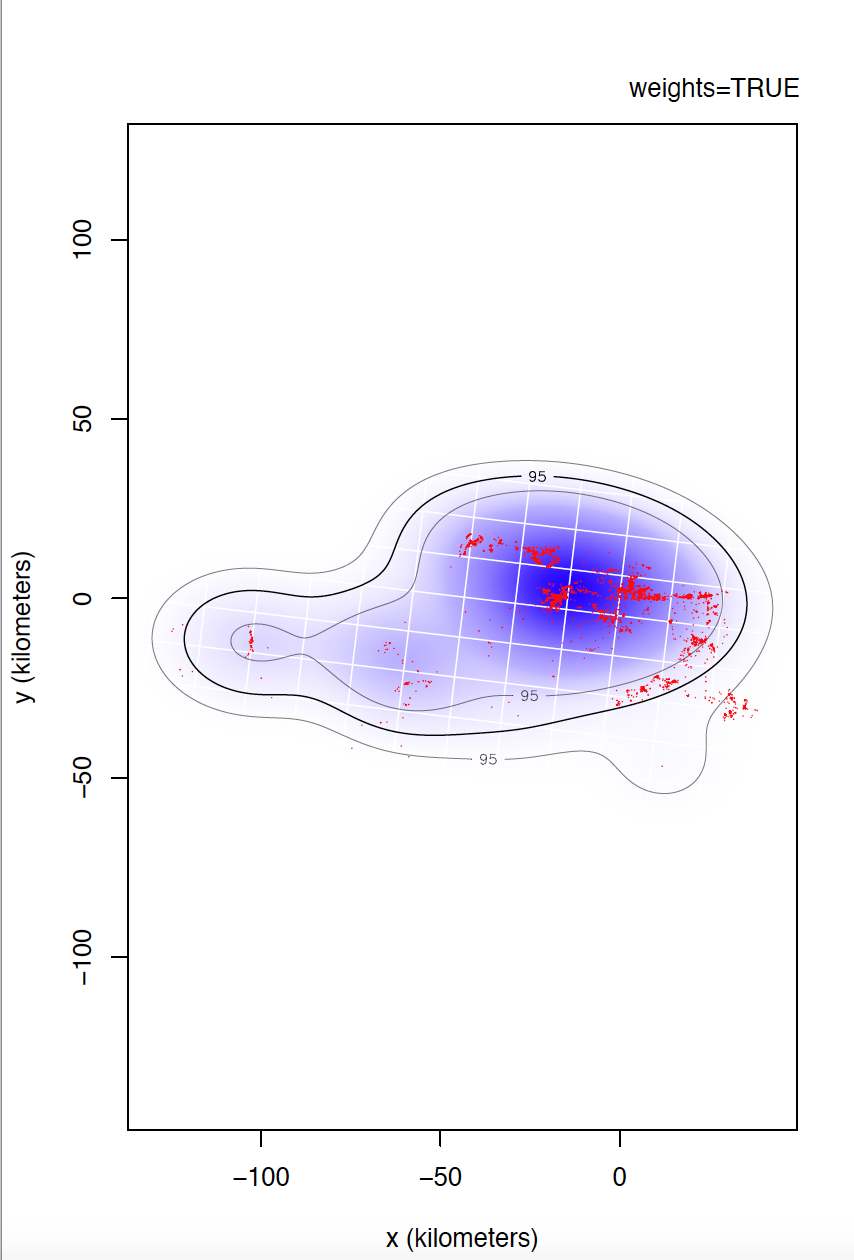
 My doubt also arises in determining whether to use the weight argument or not. As you recommended, I have classified my individuals in ascending order of DOF [area] and calculated both models weights=TRUE and weights=FALSE to check the differences between them until I find the point in which they were minimal or non-existent. But so far, I can't find that point. Individuals with lower DOF [area] may have smaller differences than individuals with higher DOF [area] or vice versa without a clear pattern in which the differences decrease as DOF [area] increases. Even in one of the individuals analyzed, the core with the highest probability of presence moves completely not using this argument. The only trend that I have been able to verify, although it is not always fulfilled, is that using weights = TRUE drifts to larger presence areas. 

At this point I start to be skeptical of whether to use the argument or not, because I'm afraid to not use it and be overestimating the area. However, applying weight=TRUE there are some individuals that I can not calculate due to processing times. 

Do you think that using weight=FALSE could lead to these overestimates? And if there is no clear pattern that allows you to choose which individuals to use with and without weights = TRUE, is there any other approach to choose it?

I would also like to ask you about how to interpret the values of the PDF. I would like to make comparisons between the probability of presence of several individuals. As I have interpreted, PDF is the one I should be using. However, the results between different individuals may have differences of several orders of magnitude for the maximum value of presence probability. This leads me to wonder if normalize to 1 all the individuals is the right thing to do to be able to compare them. Could I use the CDF for this purpose as well?

 

Thank you very much in advance!

Jorge.RP

[Christen Fleming]

Hi Jorge,

What is the duty cycling on your collars/tags?

For the slower individuals, is there progress showing when trace=TRUE? For those individuals, are there giant gaps in the data or something that could be causing that?

Are you using a more recent development version of the package from GitHub? I changed the default dt argument to be faster in some cases.

When some times are oversampled, weights=FALSE can bias the density estimate to the over sampled areas. There is an example of this given in vignette('akde') . Usually with regular duty cycling, this is not an issue, because there are no particular times/areas that are oversampled.

What kind of comparison are you trying to make with the PDF? I don't quite understand the intention.

Best,

Chris

[Jorge .Rodríguez Pérez]

Hi Chris, 

My tags are configured to collect information at 5-minute intervals, with winter periods in which the collection was limited to every 30 minutes in order to save battery and suppression of night records. 

Progress do shows when trace=TRUE and I am using the most recent version available.  With these slower individuals, what happens is that after a long time of processing, the progress of trace=TRUE stops appearing, as if the program were hanging, forcing me to restore session. It could even be a problem of the capacity of my computer, although in others that I have tested it does not seem to work either. 

As far as I can tell, or interpret, neither do I have giant gaps in the data for the majority of birds. Yet, the example given in vignette ('akde') is what may be happening in the individual who changes the core with the highest probability of presence. Did not know about this fact, but looking at the sampling of this individual, it makes sense to me.  

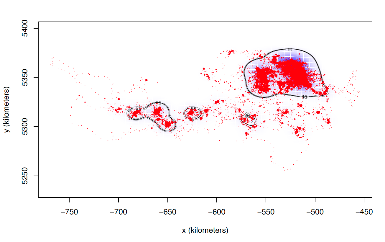
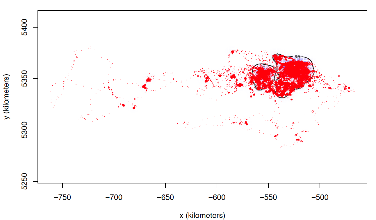
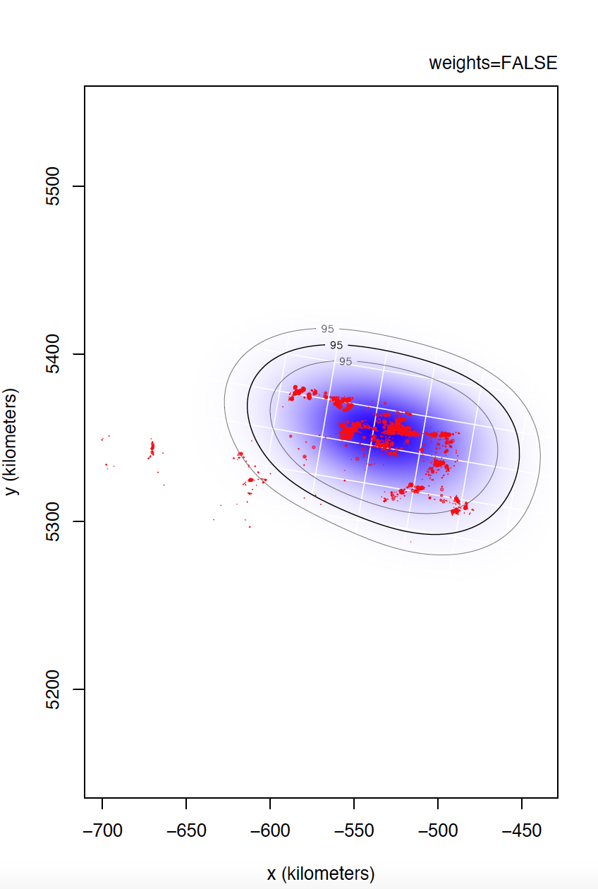
The only explanation I can think of is that these individuals I can not calculate seem to match those who make larger dispersive flights. I attach two images of two individuals calculated with weights=FALSE. Most of the locations are in the same area, while these individuals tend to make dispersive flights that can last several days (or even months) through areas that they never revisit. Most individuals with whom I cannot calculate the model with weights = TRUE perform this type of flight, in addition to being the ones with the highest numbers of data, and I do not know if that can affect the processing time and number of calculations. 

Anyway, I still have the doubt of the cases in which I have calculated both models weights = TRUE and weights = FALSE that present differences between them although not excessively large. So far, I have not found a justification that allows me to follow the same criteria to choose one or the other and that is met in all individuals.  

Regarding the use I want to give to the PDF, my intention is to obtain a final raster with the probability of joint presence for all my individuals. I have tried to use the mean function and it seems that I get the results I was looking for. My doubt arises because the maximum value of presence can have differences of several orders of magnitude between individuals and I do not know if they are comparable to each other. For example, the pixel with the highest probability of presence found in the core of individual A's home-range may have the same value as a marginal zone pixel of individual B's home-range. For individual A, that is the area with the greatest probability of presence, but I do not know if it is comparable to the area of greatest presence of individual B. As my ultimate goal is to obtain a map with the use of the territory of the population as a whole, I do not know if it makes sense to first normalize the camping areas for each individual and then obtain the joint result in a GIS environment, or if the mean function serves my goal. I also have the doubt if instead of the PDF for this purpose, I can use the CDF as it already have the accumulated probability. 

Thank you for the quick response!

Jorge.RP

[Christen Fleming]

Hi Jorgen,

Having a 5-minute interval in spring-fall and 30-minute interval in the winter could definitely bias the yearly range estimate against the wintering areas with weights=FALSE. If you can send me an example dataset that is problematic, then I can take a look at what the issue is. At least for simple cases like this, it's formally possible to assign one weight-per-time to the 5-minute data and one weight-per-time to the 30-minute data, and then to very quickly optimize the two weights versus the current code, which is much more flexible (and more optimal) but optimizes one weight for each time (100k in your case). I could potentially code that up without too much trouble.

If you want a map of the territory of the entire population, then currently you will want to calculate the individual UDs on a consistent grid and then to feed them into mean(), which was recently updated on GitHub to include population CIs derived from a hierarchical model. The output population distribution estimate will have both a PDF and CDF computed.

Best,

Chris

[Jorge .Rodríguez Pérez]

Hi again Chris, 

 Thank you very much for the involvement. 

I send you two datasets (individual 6529 and individual 5433) with which I have problems calculating the models with weights=TRUE. It seems to me, especially after your explanations, that these two individuals are problematic because of inconsistencies in sampling. You can see that for none of them the duty cycling corresponds exactly to the configuration that would correspond to it, since these are probably the two individuals with the worst dataset quality. For both cases, I interpret that weights=TRUE attribute as necessary. 5433 took me approximately 48 hours to obtain it, while for 6529 I had to stop the process after more than 72 hours, with trace=TRUE returning only a single record after that time. 

I also give you an example of an individual (7228) with a much more consistent sampling, but also with some irregularities according as I can understand. For this case, weights=TRUE is not a problem, performing the process in about 5 hours. What surprises me is that being approx. twice as many records, there are those temporal differences. 

For this last individual, weights=TRUE and weights=FALSE has different results, although relatively acceptable. For the current project I am doing, assuming weights=FALSE in most individuals seems reasonable to me considering the processing time, but I am not sure that this is the case either. Do you think those differences can be assumed, especially considering that it is for a master's thesis, with the future aim of using weights=TRUE for all cases?  

Regarding the population map, yes, I had used the mean function and the result is what I wanted to achieve. But I still have the doubt of whether I wanted to compare two individuals with each other, the values of the PDF are still comparable even having the maximum values of probability several orders of magnitude of difference. 

Again, thank you very much for the involvement and I hope to not be bothering you!

Here is the link to the datasets: https://drive.google.com/drive/folders/1Q7EVKHFYKFU7boc6Bb-tS8cvP7CyRvAV?usp=sharing

 Jorge.RP

[Christen Fleming]

Hi Jorge,

Just to give a progress update, I'm analyzing the most problematic dataset (6529) and there are many sub-minute sampling intervals down to 10 seconds. Because of the tiny sampling intervals, this dataset requires either a location-error model or some thinning. See https://www.biorxiv.org/content/10.1101/2020.06.12.130195v2.full and vignette('error') .

The data seem to be of the e-obs variety, but are missing the usual e-obs horizontal accuracy estimate.

Therefore, I'm fitting a model with with the HDOP values and a prior as in the referenced vignette and I will see how that goes. But calibration data would be preferable.

Right now I'm running some tests to try to see what good parameters are here, and what I may need to tweak to have cases like this work out of the box. I think the issue is that there is more than a year of data, but also the sampling intervals frequently get all the way down to 10 seconds, but also they do this without any clear structure, as the median time interval isn't even a multiple of 10 seconds. For small datasets, fast=FALSE, PC='direct' is what I would normally do in a case with totally irregular sampling like this, but this dataset is almost too big for that method and fast=TRUE relies on time discretization for an FFT. I am still working on it, though, and will have something for you soon.

I'm not sure what you mean about comparing individuals. Do you want to do something like evaluate the likelihood of one individual's locations based on the other individual's distribution?

Best,

Chris

[Jorge .Rodríguez Pérez]

Hello again Chris, 

 

Seriously, thank you very much for the involvement.  

I could not confirm you if individual 6529 is the most problematic. I would even venture to say that individual 5433 has even more irregular sampling. I can't compare individual 6529 yet, but take a look at the differences between weights=TRUE and FALSE for individual 5433. 

Yes, data is of e-obs variety, specifically first-generation tags. As you said,  e-obs horizontal accuracy estimateis is "missing". According to the paper you are quoting, as.telemetry imports the values of e-obs horizontal accuracy estimate as HDOP values, so I renamed this variable like this, is not that horizontal accuracy estimate is missing. I should have tell about this. Could this have caused more problems than benefits? Anyway, I upload to the same link the datasets directly extracted from movebank without any filter if that can help. 

Regarding the last part, sorry for being a pain. On the one hand, I want to compare the probability of presence for the entire population with other risks maps. Mean function is what I am using to obtain distribution raster maps, and works fine for what I want. On the other hand, I also want to compare the risks presented by each individual. This is where I wonder if the maximum probability values of presence are comparable to each other even with values of different order of magnitude. If the values for individual A at the core of its range are the same as the values for individual B in a marginal zone of its distribution, does it mean that these values are comparable and so, that the maximum probability of presence for A in its core area is less than the maximum probability that B would have in its core?  Could the data be first normalize in order to  make it comparable to each other and that the values of the core area of A are equal to the values of the core area of B?. All this assuming I use the PDF. That is why at first, I thought about using the CDF. 

Thank you so much 

Jorge. 

[Christen Fleming]

Hi Jorge,

I would construct a different prior for eobs horizontal accuracy estimates, but otherwise it is not very different from what I did to investigate.

I've figured out what is happening with your data. Attached is a plot of the sampling intervals on a log scale:

The default option is selecting dt=10 seconds, as that isn't too far below the median sampling interval, but it is too slow for over a year of data (as the discretized grid would be over a year in 10 second increments), and the 10 second intervals are also not super common. I've highlighted the most frequent sampling intervals and 5 minutes looks like a good choice for dt because it is the smallest of the most frequent sampling intervals and because the larger common sampling intervals are all divisible by 5 minutes. So I tried dt=5 %#% 'min' and the calculation was very quick. I also subsampled the data a few times and compared that output with fast=FALSE (which involves no discretization) to confirm that it was accurate.

If I understand you correctly, evaluating the probability density of a hazard would be useful, because it would be proportional to the chance of encountering the hazard at that location. In that sense it is a better proxy for risk than the CDF would be.

Best,

Chris

[Elena Bravo]

Hi Chris, 

I was following your lasts comments and wanted to ask you something. Would you see fit to establish dt=5 min for this two different dataset? the ylines that I establish here consist in 5min intervals. The y axe "dif" refers to the log10 values of the time intervals.

With this dt my dataset runs a lot faster, but I am not sure if, for example in this first plot that would be correct. Thanks for your imput in advanced!

[Christen Fleming]

Hi Elena,

If I understand the plots, the most frequent interval is 10^1 minutes and the other frequent intervals are multiples of 10 minutes, so dt = 10 %#% 'min' should suffice. But since 5 minutes is half of 10 minutes, that should just improve the discrete approximation.

Best,

Chris

[Ben Carlson]

Hi Chris,

This is a very useful figure for examining sampling intervals. Could you let us know how you produced it?

Thank you!

Ben

--
You received this message because you are subscribed to the Google Groups "ctmm R user group" group.
To unsubscribe from this group and stop receiving emails from it, send an email to ctmm-user+...@googlegroups.com.
To view this discussion on the web visit https://groups.google.com/d/msgid/ctmm-user/1d87f272-f73a-4261-8829-04a838805518n%40googlegroups.com.

[Christen Fleming]

Hi Ben,

DT <- diff(DATA$t) # get sampling intervals
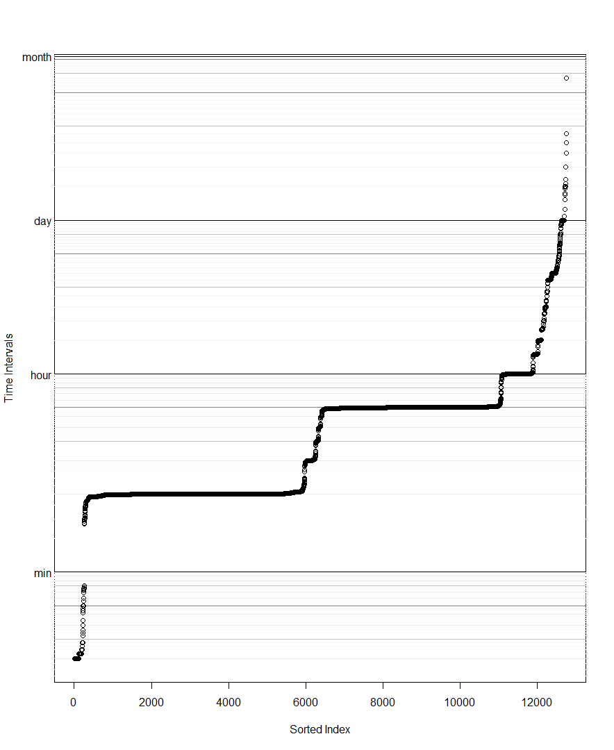
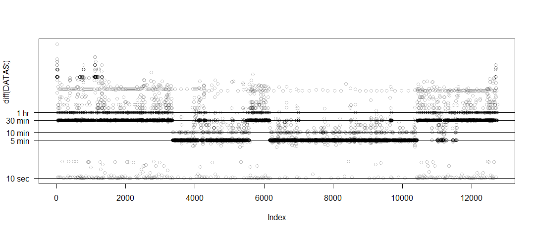
DT <- DT[DT>0] # remove for log scale
DT <- sort(DT) # Beth's idea

plot(DT,log='y',yaxt='n',ylab='diff(time)',col=rgb(0,0,0,1/4))

# example horizontal line with labeled tick
abline(h=1 %#% 'hr')
axis(side=2,at=1 %#% 'hr',label='1 hr',las=2)

I'd make a function for this if I could figure out how to reliably automate some of the modal interval estimation/selection.

Best,

Chris

[Francisco Castellanos]

Christen,

Thanks for sharing this with the group. I've been using a function in the package tlocoh to look at the sampling intervals, I don't think it's as good as the lines of code you just shared but still I thought I'd share: 

library(tlocoh)

lxy.plot.freq(DF, delta.by.date= T, time.unit="hour") 

Regards,

Francisco

To view this discussion on the web visit https://groups.google.com/d/msgid/ctmm-user/cf38be5e-a423-4db6-9972-b320655b7f41n%40googlegroups.com.

[Christen Fleming]

I pushed a basic function dt.plot() to the development branch. It makes a plot like this from (potentially multiple) datasets:

with lines at common intervals, and you can check the 5-minute interval here with something like abline(h=5%#%'min',col='red') .

locator() doesn't seem to be working for me in RStudio.

Best,

Chris