IC-QMMM with single charge in front of a metal plane: open boundary corrections

[Katharina Doblhoff-Dier]

Dear CP2K community,

I am confused about the IC-QMMM method as implemented in CP2K. I am not 100% sure whether my question is related to my misunderstanding of the method (as implemented) or on how to use it.

Originally, my confusion came from my not-understanding of the parameter V_0 (i.e., EXT_POTENTIAL in the CP2K implementation): In periodic boundary conditions, this parameter does not seem to make much sense to me: Depending on the average potential in the quantum region, defining V_0 will make the charge Q on the metal adapt in such a way that the average potential in the cell is zero (I know that the latter is logic, but in view of this, the physical meaning of V_0 becmes unclear to me):

Alternatively, if a charge is put into the QM part (e.g. an H2+) and V0 is adjusted such that the total charge Q on the metal is exaclty -1, a spurious field will result over the cell (due to Ewald summation) and again, V_0 does not have an obvious physical meaning.

Considering that the periodic boundary conditions lead to lots of spurious stuff, I then tried to go to MT boundary corrections or the IMPLICIT poisson solver as implemented in CP2K. This gave me the following results (note that I shifted the green and the blue curve by 0.4V for better comparison)

red:      IMPLICIT poissn solver with Neumann BC at z=0 and z=60 and homogeneous Dirichlet BC at z=30

green:  MT (Martyna-Tuckerman) poisson solver (shifted by 0.4V)

blue:    normal Ewald summation (shifted by 0.4V)

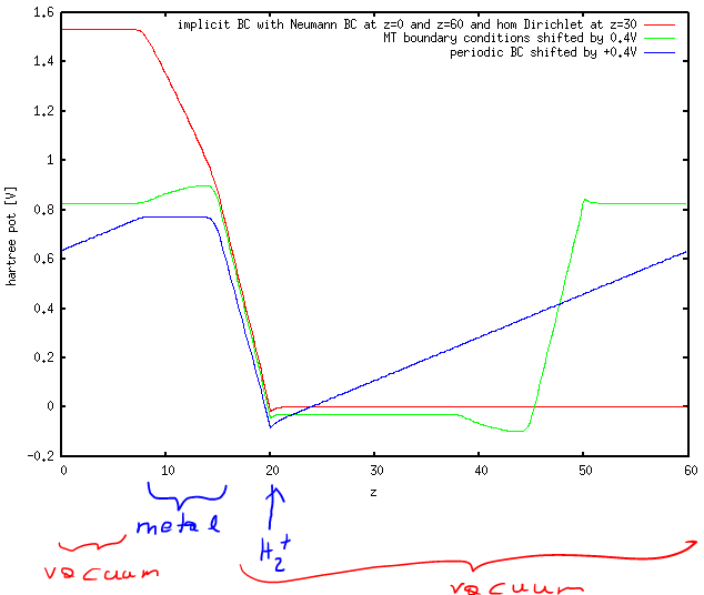
The corresponding V_0 (optimized such that Q=-1) were 1.11V for IMPLICIT boundary conditions, 1.24V for MT boundary conditions and -0.37V for periodic boundary conditions. While for periodic boundary conditions (blue line) this can be seen to correspond to the potential in the metal part, this is not the case for MT boundary conditions (green), where the potential in the metal varies from about -0.4 to -0.5 (remember that I shifted the curves by 0.4 volt) and for IMPLICIT boundary conditions. Overall, to me, it looks as if the IC-QMMM method was ignoring the boundary conditions and optimizing the charges for the periodic boundary conditions and then keeping them fixed no matter what I set as POISSON_SOLVER. In the MT boundary condition case (geen) we can thus see the influence of the charges shieding the (spurious) field in periodic boundary conditions (hence the slope in the metal part, which has the same slope as the average field in the periodic solver).

Finally, I decided that, in principle, it should be possible to find an energy minimum when Q_image=-Q_QM (as also shown in the original paper by Siepmann and Sprik). With none of the boundary conditions could I find this minimum correctly. However, here comes my non-understanding of Eq. 4 in the paper by Golze, Iannuzzi, ..., and Hutter (https://pubs-acs-org.ezproxy.leidenuniv.nl:2443/doi/10.1021/ct400698y) into play: Here, the energy is written as:

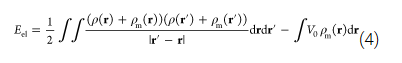
I would have thought this to be a grand canonical energy (grand canonical only in the charges on the metal) expression, where the last term accounts for the -N_i*mu_i term. Again, this does not seem physical to me if I think of a capacitor (or a charge+image charge in a box that is periodic in x and y, as I would then expect a correction for the charges in the QM region too (unless the vacuum potential on the QM side is zero and open boundary conditions are used, but likely this is wrong and this may be where my entire confusion starts.

So summarizing, this boils down to a few questions:

1.) can the IC-QMMM method be combined with poisson solvers other than periodic? If so, how? I simply set the poisson solver in the MM and the DFT part.

2.) What do I need to do in order to find an energy minimum for Q_image=-Q_QM?

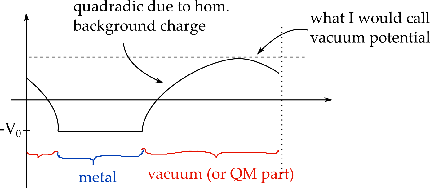
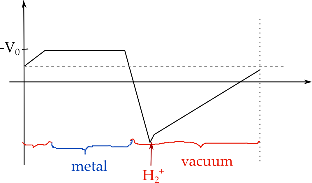
3.) What is the meaning of V_0 and why is it substracted in the energy expression.

Any physical insight is appreciated!

Thank you and best regards,

Katharina

[Dorothea Golze]

Hi Katharina,

I am not sure if I understand your question correctly and what your computational setup is.

The basic electrostatic consideration is that the potential should be constant within a conductor. If no external potential is applied, the electrostatic potential is zero within a metal, i.e., V_0=0. That is the default. It can be also set to another value  in principle, e.g., maybe to approximate the application of a potential to an electrode. But it seems that's not what you want to do here. Note that the IC-QM/MM does not introduce actual charges, only image charges. You can run with the normal periodic solver when you have a (neutral) molecule on top of the metal (MM).

If you have a charged system in the QM part, then you need a solver like MT, like in a standard QM calculation.

Best regards,

Dorothea

--
You received this message because you are subscribed to the Google Groups "cp2k" group.
To unsubscribe from this group and stop receiving emails from it, send an email to cp2k+uns...@googlegroups.com.
To view this discussion on the web visit https://groups.google.com/d/msgid/cp2k/5774878e-630c-4699-a67e-5040897c1b2do%40googlegroups.com.

[Katharina Doblhoff-Dier]

Dear Dorothea,

Thank you for your answer. 

I am not sure if I understand your question correctly

 

On the longer run, we are interested in describing an electrolyte above a metal surface and using a charge imbalance to create a potential drop at the interface very much as one would do in a pure DFT calculation, but then withouth the need to describe the metal quantum mechanically. I know that this is not the original idea behind the image charge method as implemented in cp2k, but I thought it may offer a work around. So to understand how things work, I simply considered an H2+ molecule above a surface. This is similar to the model system used by Siepmann and Sprik in their 1995 publication, just that they used an MM point charge above a metal. In principle, it should be possible to determine V_0 from the condition that the energy should be minimized, and the resulting counter charge should exactly cancel the charge in front of the metal.

and what your computational setup is.

I paste here an example of the input that I used with MT boundary conditions. The resulting plot for the Hartree-potential (obtained using  &V_HARTREE_CUBE and then averaging over x and y to get a plot over z) is shown in the third image in my original post (green line).

As you can see, I simply adapted the input file from the GUA example on the web, by replacing the GUA in the xyz file by H2, setting the DFT charge to 1 and changing the poisson solver in the DFT and MM part. The potential EXT_POTENTIAL was determined by running 2 calculations with changing EXT_POTENTIAL_1 and EXT_POTENTIAL_2, and then determining EXT_POTENTIAL_3 by requiring that the resulting charge should be -1 and assuming a linear relationship (which for this system is perfectly followed, giving me a total charge on the metal of -1)

-----------------Begin sample input file using the MT poisson solver------------------

&FORCE_EVAL
  METHOD QMMM
  &DFT
    CHARGE 1
    LSD
    BASIS_SET_FILE_NAME BASIS_MOLOPT
    POTENTIAL_FILE_NAME GTH_POTENTIALS
    &POISSON
      &EWALD
        EWALD_TYPE ewald
        ALPHA .44
        GMAX 21
      &END EWALD
      POISSON_SOLVER MT
      PERIODIC XY
    &END POISSON
    &MGRID
      COMMENSURATE
      CUTOFF 300
      NGRIDS 5
    &END MGRID
    &QS
      METHOD GPW
      EXTRAPOLATION ASPC
      EXTRAPOLATION_ORDER 3
    &END QS
    &SCF
      MAX_SCF 300
       SCF_GUESS ATOMIC
     # SCF_GUESS RESTART
      EPS_SCF 1.0E-6
      &OT
        PRECONDITIONER  FULL_SINGLE_INVERSE
        MINIMIZER DIIS
      &END
    &END SCF
    &XC
      &XC_FUNCTIONAL PBE
      &END XC_FUNCTIONAL
        &VDW_POTENTIAL
          DISPERSION_FUNCTIONAL PAIR_POTENTIAL
          &PAIR_POTENTIAL
           TYPE DFTD3
           CALCULATE_C9_TERM .TRUE.
           REFERENCE_C9_TERM
           PARAMETER_FILE_NAME dftd3.dat
           REFERENCE_FUNCTIONAL PBE
           R_CUTOFF [angstrom] 16.0
          &END PAIR_POTENTIAL
        &END VDW_POTENTIAL
    &END XC
    &PRINT
     &V_HARTREE_CUBE
     &END
    &END
  &END DFT

  &MM
    &FORCEFIELD
      &CHARGE
        ATOM Au
        CHARGE 0
      &END CHARGE
      &CHARGE
        ATOM H
        CHARGE 0
      &END CHARGE

      &SPLINE
       EPS_SPLINE 1.E-5
       #EMAX_SPLINE 2.0
      &END

       &NONBONDED
        &EAM
          atoms Au Au
          PARM_FILE_NAME Au.pot
        &END EAM


       &LENNARD-JONES
          atoms Au H
          EPSILON 0.0
          SIGMA 3.166
          RCUT  15
       &END LENNARD-JONES

       &LENNARD-JONES
         atoms H H
         EPSILON 0.0
         SIGMA 3.166
         RCUT 15
       &END LENNARD-JONES

      &END

    &END FORCEFIELD

    &POISSON
      &EWALD
        EWALD_TYPE ewald
        ALPHA .44
        GMAX 21
      &END EWALD
      POISSON_SOLVER MT
      PERIODIC XY
    &END POISSON
  &END MM

  &QMMM
    CENTER NEVER
    &CELL
      ABC [angstrom]   34.6055 29.9693 60.0
      PERIODIC XY
    &END CELL

    &QM_KIND H
     MM_INDEX 577..578
    &END QM_KIND

    &IMAGE_CHARGE
     EXT_POTENTIAL 1.24534
     MM_ATOM_LIST 1..576
     WIDTH 3.5
    &END IMAGE_CHARGE

    &PRINT
     &IMAGE_CHARGE_INFO
     &END
    &END

  &END QMMM

  &SUBSYS
    &CELL
      ABC [angstrom]   34.6055 29.9693 60.0
      PERIODIC XY
    &END CELL
    &TOPOLOGY
      COORD_FILE_NAME Au_gua_image_dampFunc-opt.xyz
      COORDINATE xyz
    &END
    &KIND H
      BASIS_SET DZVP-MOLOPT-SR-GTH
      POTENTIAL GTH-PBE-q1
    &END KIND

  &END SUBSYS
&END FORCE_EVAL

&GLOBAL
  PROJECT Au_gua_image_dampFunc
  RUN_TYPE energy
&END GLOBAL

-----------------End sample input file using the MT poisson solver------------------

>If you have a charged system in the QM part, then you need a solver like MT, like in a standard QM calculation.

Yes, I would have thought, that this is what I am doing, but the resulting plot for the hartree potential looks strange (shielding charges in the metal, leading to a potential gradient in the metal instead of a constant) and I cannot seem to find an energy minimum, when the potential is chosen such, that the image charge is exatly shielded, which was one of the test systems in the Siepmann Sprik paper (https://aip.scitation.org/doi/abstract/10.1063/1.469429).

I guess the latter is my main issue, as we will depend heavily on the energies. (Hence I need to understand what they contain)

Thank you for your help,

Katharina

[Katharina Doblhoff-Dier]

Dear Dorothea,

To break a complex problem down: Should I consider it a bug, that I get non-constant potentials in the plot of the hartree energies, when using MT or implicit BCs and that potential in the metal does not match EXT_POTENTIAL? (see plot below - also posted in the original question) Or is there a good reason for this behavior?

red:      IMPLICIT poissn solver with Neumann BC at z=0 and z=60 and homogeneous Dirichlet BC at z=30

green:  MT (Martyna-Tuckerman) poisson solver (shifted by 0.4V)

blue:    normal Ewald summation (shifted by 0.4V)

Thank you for your help!

Best regards,

Katharina

[Dorothea Golze]

Dear Katharina,

in short, it is very likely no bug; I think the basic problem is that you try to run a periodic DFT calculation for a charged system.
The constant potential condition is a hard constraint for the average. I tested with the standard periodic solver (for periodic systems) and the MT solver (for a cluster-type of approach).

I don't have it in the paper, but in my thesis, I have an example, where I placed an ion above a slab (Figure 3.7 page 31, https://www.zora.uzh.ch/id/eprint/116638/)

For the MT solver, I have the suspicion you are not applying this solver correctly, which can lead to technical artifacts. You need lots of vacuum around your system since you also specified a periodic cell, this seems not to be the case. I suggest to test the MT solver for a single molecule (DFT only) first to get a feeling how much vacuum you need, i.e., to converge out the cell size and how this solver behaves.

Best regards,

Dorothea

--
You received this message because you are subscribed to the Google Groups "cp2k" group.
To unsubscribe from this group and stop receiving emails from it, send an email to cp2k+uns...@googlegroups.com.

To view this discussion on the web visit https://groups.google.com/d/msgid/cp2k/168440d5-5b57-4075-900e-876a99f8e437o%40googlegroups.com.

[Dorothea Golze]

Dear Katharina,

I just ran a quick test for the EXT_POTENTIAL keyword. System: small organic molecule on top of gold (charge-neutral periodic system using standard periodic solver).  The keyword still seems to work as intended: when preparing a plane-averaged plot in z-direction, the potential is not zero in the region of the metal, but the value defined by EXT_POTENTIAL. I can send you my example input files; feel free to contact me directly (dorothe...@aalto.fi).

Best regards,

Dorothea