Differences between rstanarm and brms?

[Travis Riddle]

Hi all,

I've come across some differences between rstanarm and brms, that I'm not able to explain. I hope someone here can tell me why I'm seeing these behaviors. Below is a reproducible example:

library(languageR) #for data
library(rstanarm)
library(brms)
library(dplyr)
library(ggplot)
library(tidyr)

stan.pen <- stan_lmer(RT ~ list*priming + (priming|subjects) + (1|items), data=splitplot, 

                      prior=normal(0,250), prior_intercept=normal(500,200))

p <- c(set_prior('normal(0,250)', class='b'),

       set_prior('normal(500,200)', class='Intercept', coef=''))

brm.pen <- brm(RT ~ list*priming + (priming|subjects) + (1|items), 

               data=splitplot, prior=p)

As far as I can tell, those two models should be the same, but they are apparently not.

newdat <- expand.grid(list = rownames(table(splitplot$list)),

                      priming = rownames(table(splitplot$priming)),

                      subjects='0',

                      items = rownames(table(splitplot$items)))

temp <- as.data.frame(

  rstanarm::posterior_linpred(stan.pen, re.form = NA, 

                    newdata = newdat, allow_new_levels=T)) #the linear predictor

temp$sample <- seq(1, length(temp$`1`))

newdat$index <- as.character(seq(1, length(newdat$list)))

temp %>%

  gather(index, prediction, -sample) %>%

  left_join(newdat) %>%

  group_by(list, priming) %>%

  summarise(est = mean(prediction), #mean of the linear predictor

            lower = quantile(prediction, .025),

            upper = quantile(prediction, .975)) %>% #upper and lower 95% uncertainty intervals

  mutate(model='rstanarm') -> plot.dat 

temp <- as.data.frame(

  brms::posterior_linpred(brm.pen, re.form = NA, 

                              newdata = newdat, allow_new_levels=T)) #linear predictor

temp$sample <- seq(1, length(temp$`V1`))

newdat$index <- as.character(paste('V', seq(1, length(newdat$list)), sep=''))

temp %>%

  gather(index, prediction, -sample) %>%

  left_join(newdat) %>%

  group_by(list, priming) %>%

  summarise(est = mean(prediction), #mean of the linear predictor

            lower = quantile(prediction, .025),

            upper = quantile(prediction, .975)) %>% #upper and lower 95% uncertainty intervals

  mutate(model='brms') %>%

  rbind(plot.dat) -> plot.dat

ggplot(plot.dat, aes(x=list, y=est, group=model, color=model)) +

  geom_point(position=position_dodge(width=.5)) + 

  geom_errorbar(aes(ymin=lower, ymax=upper), position=position_dodge(width=.5)) +

  facet_wrap(~priming)

This produces the following figure:

So it seems the mean is correct, but the uncertainty intervals do not match. Why not?

I've looked at some of the actual parameters estimated, and I think there's some differences in the covariance matrix:

stan.df <- data.frame(stan.pen)
brm.df <- data.frame(brm.pen)


df <- data.frame(model = c(rep('rstanarm', 4000),
                           rep('brms', 4000)),
                 sample = c(seq(1:4000), seq(1:4000)),
                 intercept = c(stan.df$X.Intercept., brm.df$b_Intercept),
                 b_listlistB = c(stan.df$listlistB, brm.df$b_listlistB),
                 b_primingunprimed = c(stan.df$primingunprimed,
                                       brm.df$b_primingunprimed),
                 b_list_priming = c(stan.df$listlistB.primingunprimed,
                                    brm.df$b_listlistB.primingunprimed),
                 sigma = c(stan.df$sigma, brm.df$sigma),
                 sigma.items_int = c(stan.df$Sigma.items..Intercept...Intercept..,
                                     brm.df$sd_items__Intercept),
                 sigma.subjects_int = c(stan.df$Sigma.subjects..Intercept...Intercept..,
                                        brm.df$sd_subjects__Intercept),
                 sigma.subjects_priming.int = c(stan.df$Sigma.subjects.primingunprimed..Intercept..,
                                                brm.df$cor_subjects__Intercept__primingunprimed),
                 sigma.subjects_priming = c(stan.df$Sigma.subjects.primingunprimed.primingunprimed.,
                                            brm.df$sd_subjects__primingunprimed))

df %>%
  gather(parameter, value, intercept:sigma.subjects_priming) %>%
  ggplot(aes(x=value, group=model, color=model)) +
  geom_density() +
  facet_wrap(~parameter, scales='free')

Sorry if I've missed something obvious in the documentation. What explains this behavior? Even if I'm misunderstanding the parameters (or something), I would expect the function `posterior_linpred` to perform identically in these situations, unless I've misspecified the model...

[Paul Buerkner]

Strange, I would expect the same behavior from posterior_linpred, as well.

Based on the plot you provided, it looks like the "sigma" parameters estimated by rstanarm are huge as compared to those of brms. This looks suspicious to me. Are you sure the rstanarm model sampled correctly?

--
You received this message because you are subscribed to the Google Groups "brms-users" group.
To unsubscribe from this group and stop receiving emails from it, send an email to brms-users+unsubscribe@googlegroups.com.
To post to this group, send email to brms-...@googlegroups.com.
To view this discussion on the web visit https://groups.google.com/d/msgid/brms-users/4c5e36a1-dd48-497c-8419-8680f2f3985d%40googlegroups.com.
For more options, visit https://groups.google.com/d/optout.

[Paul Buerkner]

When I run the brms model and call marginal_effects(brm.pen), I get the above plot.

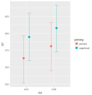
The lines pretty much look like the blue lines in your plot, which you labled as belonging to rstanarm.

[Paul Buerkner]

I get it now. In brms, the argument is called re_formula not re.form. This is unfortunate and I will introduce the re.form alias in the next version of brms.

[Travis Riddle]

Ah! This is great. Thanks a lot Paul. So the values given by posterior_linpred in brms included all random effects? 

Also, amazing work on the package. 

[Paul Buerkner]

Yes they included the uncertainty of the random effects.

--
You received this message because you are subscribed to the Google Groups "brms-users" group.
To unsubscribe from this group and stop receiving emails from it, send an email to brms-users+unsubscribe@googlegroups.com.
To post to this group, send email to brms-...@googlegroups.com.

To view this discussion on the web visit https://groups.google.com/d/msgid/brms-users/197e08f8-24f9-41bd-a0c1-5f0886fc5d29%40googlegroups.com.

[Travis Riddle]

Hello again,

I've still been running into some differences between rstanarm and brms. Unfortunately, I can't reproduce these differences with a publicly available dataset (at least, none that I know of), so I've shared a sample of the data I'm working with. As the models take some time to run and I had issues with divergent transitions (note the high adapt_delta values below), I've also shared the two models (brms.rdata; rstanarm.rdata).

The code used to fit the models is as follows:

library(rstanarm)
library(brms)
library(dplyr)
library(ggplot2)


testing_data <- read.csv('testing_data.csv')


p <- c(set_prior('normal(2,2)', class='Intercept', coef=''),
       set_prior('normal(0,1)', class='b'))
 


m.brm <- brm(gpa ~ Condition*Ethnicity + (1|ID) +
               (Condition*Ethnicity|site), data=testing_data,
             control=list(adapt_delta=.9999, max_treedepth=15), prior=p)
m.rstanarm <- stan_glmer(gpa ~ Condition*Ethnicity + (1|ID) +
                           (Condition*Ethnicity|site),
                         prior_intercept=normal(2,2), prior=normal(0,1),
                         data=testing_data, adapt_delta = .9999999)

looking at the posterior estimates for the experimental cells (condition & ethnicity):

There are some differences in the mean for each of these parameters, but they're sufficiently small that I suspect they would converge in the limit. The variance, however, I have no explanation for, and seems much too great to be due to sampling variability (plus, this recurs with new fits and different samples of the data).

summary(m.brm)

 ...(truncated)...


Population-Level Effects:

                                  Estimate Est.Error l-95% CI u-95% CI Eff.Sample Rhat

Intercept                             2.35      0.29     1.73     2.88       1504 1.00

ConditionTreatment                    0.20      0.30    -0.40     0.79       1011 1.00

EthnicityWhite                        0.84      0.30     0.16     1.38       1377 1.00

ConditionTreatment:EthnicityWhite    -0.24      0.39    -0.97     0.55       1223 1.00




Family Specific Parameters:

      Estimate Est.Error l-95% CI u-95% CI Eff.Sample Rhat

sigma     0.44      0.01     0.42     0.47       4000 1.00




Samples were drawn using sampling(NUTS). For each parameter, Eff.Sample

is a crude measure of effective sample size, and Rhat is the potential

scale reduction factor on split chains (at convergence, Rhat = 1).

summary(m.rstanarm)[1:4,c(1,3,4,8,9,10)]



                                        mean        sd       2.5%     97.5% n_eff     Rhat

(Intercept)                        2.3478353 0.2047021  1.9469587 2.7573228   552 1.003772

ConditionTreatment                 0.2405582 0.2505187 -0.2488431 0.7221305   472 1.008159

EthnicityWhite                     0.9094795 0.2283877  0.4650232 1.3454927   465 1.005876

ConditionTreatment:EthnicityWhite -0.3137621 0.3100872 -0.9194833 0.2908425   385 1.005505

Any insight would be extremely valuable to me. Thanks,

-Travis

On Monday, November 20, 2017 at 1:47:12 PM UTC-5, Paul Buerkner wrote:

Yes they included the uncertainty of the random effects.

Am 20.11.2017 19:42 schrieb "Travis Riddle" <rid...@gmail.com>:

Ah! This is great. Thanks a lot Paul. So the values given by posterior_linpred in brms included all random effects? 

Also, amazing work on the package. 

On Monday, November 20, 2017 at 7:56:54 AM UTC-5, Paul Buerkner wrote:

I get it now. In brms, the argument is called re_formula not re.form. This is unfortunate and I will introduce the re.form alias in the next version of brms.

--
You received this message because you are subscribed to the Google Groups "brms-users" group.

To unsubscribe from this group and stop receiving emails from it, send an email to brms-users+...@googlegroups.com.

[Paul Buerkner]

Thanks Travis for providing such detailed information.

The posterior-mean values of the random effects SDs of site appear to be larger in brms:

> VarCorr(m.brm)$site$sd[, "Estimate", drop = FALSE]
                                   Estimate
Intercept                         0.4496999
ConditionTreatment                0.3888073
EthnicityWhite                    0.4617288
ConditionTreatment:EthnicityWhite 0.5834659

than in rstanarm:

> VarCorr(m.rstanarm)
 Groups   Name                              Std.Dev. Corr               
 ID       (Intercept)                       0.75533                     
 site     (Intercept)                       0.27836                     
          ConditionTreatment                0.22673  -0.097             
          EthnicityWhite                    0.23986   0.085 -0.099      
          ConditionTreatment:EthnicityWhite 0.25943   0.033 -0.083 -0.184
 Residual                                   0.44043                       

I have to investigate this in more detail, but this might be the result of narrower priors on the group-level SDs of site in rstanarm as compared to brms. Since larger values of the group-level SDs imply larger variation in the population-level effects, this might explain the differences you observed.

In contrast, the SD of ID and the residual SD is pretty similar for both packages since in brms:

> VarCorr(m.brm)$ID$sd[, "Estimate"]
[1] 0.7569105

> VarCorr(m.brm)$residual__$sd[, "Estimate"]
[1] 0.4405743

similar to what we see above from rstanarm. Accordingly I would expect this to be a problem of too narrow priors of the SDs in rstanarm, but only for correlated group-level effects. Again, this conclusion is preliminary and needs to be investigated further also by the Stan Team.

To unsubscribe from this group and stop receiving emails from it, send an email to brms-users+unsubscribe@googlegroups.com.

To post to this group, send email to brms-...@googlegroups.com.

To view this discussion on the web visit https://groups.google.com/d/msgid/brms-users/50740ef1-fa8c-42c7-b027-04b736940d62%40googlegroups.com.

[Paul Buerkner]

[Travis Riddle]

Thanks Paul, this is indeed what I had suspected. I posted about this on the stan forums as well, though it was some time ago and I didn't provide data or models.

http://discourse.mc-stan.org/t/varying-variances/2476/4

As I said there when asking about the prior:

My guess would be the LKJ prior, but both packages say that zeta is set to 1 by default, and some mild adjustments to the brms model have not changed the patterns here.

But perhaps I was wrong here: in the Stan code generated by brms, I should instead adjust the sigma value of priors used here:

  target += student_t_lpdf(sd_2 | 3, 0, 10)
    - 5 * student_t_lccdf(0 | 3, 0, 10);

Though I'm not entirely clear what is going on here with the student_t_lpdf() - 5*student_t_lccdf...

Thanks,

Travis

[Paul Buerkner]

The LKJ prior ist just about the correlations not the SDs and the latter are causing the differences in our case.

target += student_t_lpdf(sd_2 | 3, 0, 10)
    - 5 * student_t_lccdf(0 | 3, 0, 10);



is simply a half-student-t prior with df = 3 and scale = 10 and only the first of the two lines is relevant for our purposes. The
- 5 * student_t_lccdf(0 | 3, 0, 10) is nothing you should worry about. It simply makes sure that Bayes factors based on brms models can be computed correctly.

--
You received this message because you are subscribed to the Google Groups "brms-users" group.

To unsubscribe from this group and stop receiving emails from it, send an email to brms-users+unsubscribe@googlegroups.com.

To post to this group, send email to brms-...@googlegroups.com.

To view this discussion on the web visit https://groups.google.com/d/msgid/brms-users/031291b7-a50f-48e3-8ddb-427a6d1eabe1%40googlegroups.com.

[Travis Riddle]

Thanks Paul. I'll try to adjust the priors and see where that leads me.

One more question based on your comment here:

I would expect this to be a problem of too narrow priors of the SDs in rstanarm, but only for correlated group-level effects

I'm not sure I understand this. Why would the width of the prior only have these consequences for correlated effects? 

To unsubscribe from this group and stop receiving emails from it, send an email to brms-users+...@googlegroups.com.

[Paul Buerkner]

My comment was just based on the observation I made for your model. Likely it is invalid in general.

I don't know for sure how rstanarm handles its group-level SD priors, but I would (as you say) expect them to be the same for correlated and uncorrelated effects.

It is possible of course, that there is a difference because of an error in their Stan code.

Let's see what the Stan team says about this problem.

To unsubscribe from this group and stop receiving emails from it, send an email to brms-users+unsubscribe@googlegroups.com.

To post to this group, send email to brms-...@googlegroups.com.

To view this discussion on the web visit https://groups.google.com/d/msgid/brms-users/70c58017-bded-48ce-99d6-7d809dec79cf%40googlegroups.com.

[Travis Riddle]

For completeness, the thread on the stan forums is here. 

My take-away is that the group-level SD is handled really differently in rstanarm, but this probably only becomes noticeable if there are relatively few groups, as in my case where there are 5.

[Paul Buerkner]

Thank you! That makes sense!

To unsubscribe from this group and stop receiving emails from it, send an email to brms-users+unsubscribe@googlegroups.com.

To post to this group, send email to brms-...@googlegroups.com.

To view this discussion on the web visit https://groups.google.com/d/msgid/brms-users/ec2671a5-831a-4f88-9a99-310d59dd7264%40googlegroups.com.