Individual Level Parameters with more than one random parameter
364 views
Skip to first unread message

Álvaro A. Gutiérrez-Vargas
Oct 18, 2021, 6:12:38 AM10/18/21
to Biogeme
Dear Michel,
Álvaro A. Gutiérrez-Vargas
PhD student at ORSTAT
KU Leuven, Belgium
https://alvarogutyerrez.github.io/
I recently started using BIOGEME, and I am trying to obtain the posterior distributions for the randomly distributed parameters (a.k.a individual-level parameters). I am aware of example number 19 where you provided an illustration for this using the MonteCarlo() function to create them. However, in my case I have two small differences with respect to said example, 1) I am working with more than one random parameter, and 2) I am working with panel data (more than one choice set per individual). Consequently, I haven't managed to produce the individual-level parameters using the example you provided.
Below you can find a script that generates a data set with two normally distributed parameters and recovers them using fitting a Mixed Multinomial Logit. However, at the very bottom of the script, I am confused with how to specify what you called "numerator" and "denominator" in the example you provided using the MonteCarlo() function (i.e. line: numerator = MonteCarlo(B_x1_RND * B_x2_RND * logprob) ### ???).
Could you please help me out with this issue, or point me towards an example/documentation part that I might possible overlook?
Could you please help me out with this issue, or point me towards an example/documentation part that I might possible overlook?
Thank you a lot for your time.
Best regards,
PhD student at ORSTAT
KU Leuven, Belgium
https://alvarogutyerrez.github.io/
# -*- coding: utf-8 -*-
#----------------------------------
#"""
Created on Tue Oct 12 10:24:06 2021
@author: Álvaro A. Gutiérrez-Vargas
"""
import pandas as pd
import numpy as np
import biogeme.database as db
import biogeme.biogeme as bio
from biogeme import models
import biogeme.messaging as msg
from biogeme.expressions import Beta, DefineVariable, bioDraws, log, MonteCarlo, PanelLikelihoodTrajectory
####----------------------------####
####---- SIMULATED DATA ----####
####---- IN ----####
####---- LONG FORMAT ----####
####----------------------------####
# Random seed for replicability
np.random.seed(777777)
N = 300 # Number of individuals
J = 3 # Number of alternatives
t = 20 # Choice sets per individual
# Individual id
id = np.repeat(range(1, N*t+1), J).reshape(N*t*J,1)
# Alternative identifier in long format
altern = np.tile(range(1,J+1),N*t).reshape(N*t*J,1)
# Attribute levels
x1 = np.random.normal(0,1,N*t*J).reshape(N*t*J,1)
x2 = np.random.normal(0,1,N*t*J).reshape(N*t*J,1)
# Random parameters
#beta_1: Normal distribution
b_1 = np.random.normal(1,0.5,N)
b_1 = np.repeat(b_1,t*J).reshape(N*t*J,1)#comformability
#beta_2: Normal distribution
b_2 = np.random.normal(1,0.5,N)
b_2 = np.repeat(b_2,t*J).reshape(N*t*J,1) #comformability
# Utility
U = b_1 * x1 + b_2 * x2
# Exp(U)
U_exp = np.exp(U)
# Denominator sum exp(U) of all alternatives
sum_exp = np.repeat(np.array([(U_exp[id==i]).sum() for i in np.unique(id)]), J).reshape(N*t*J,1)
# Probability
pbb = U_exp/sum_exp
# This generates (N*t x J) matrix with chosen alternatives using multinomial samples
choice = np.array([np.random.multinomial(1,(pbb[id==i])) for i in np.unique(id)])
# this identify the number of the selected alternative
num_choice = np.repeat(np.argmax(choice, axis=1)+1,J).reshape(N*t*J,1)
# this turn the last object into a dummy variable indicating the chosen altenative
Y = 1*(num_choice ==altern).reshape(N*t*J,1)
## long format data set
array_long = np.concatenate((id,altern,x1,x2), axis=1)
df_long = pd.DataFrame(data = array_long, columns = ['id','altern','x1','x2'])
# astype integer in order to get ride of names variables such as "x1_1.0"
df_long['altern'] = df_long['altern'].astype(int)
####----------------------------####
####---- LONG TO WIDE DATA ----####
####----------------------------####
# Reshape/Pivot long format data into Wide format required by Biogeme.
df_wide=df_long.pivot(index='id', columns='altern', values=['x1','x2'])
df_wide = df_wide.sort_index(axis=1, level=1)
df_wide.columns = [f'{x}_{y}' for x,y in df_wide.columns]
df_wide = df_wide.reset_index()
#CHOICE variable in wide format
CHOICE = (np.argmax(choice, axis=1)+1).reshape(N*t,1)
#id individuals in wide format
id_ind = np.repeat(range(1, N+1), t).reshape(N*t,1)
#id choice situation of individual n in wide format
id_choice_situation_of_individual_n = np.tile(range(1,t+1),N).reshape(N*t,1)
## long format data set
id_plus_choice_wide = pd.DataFrame(data =np.concatenate((id_ind,id_choice_situation_of_individual_n,CHOICE), axis=1),
columns = ['id_ind','id_choice_situation_of_individual_n','CHOICE'])
df = id_plus_choice_wide.join(df_wide)
####----------------------------####
####---- BIOGEME DATABASE ----####
####----------------------------####
database = db.Database('MMNL', df)
database.panel("id_ind")
# The following statement allows you to use the names of the variable
# as Python variable.
globals().update(database.variables)
# Parameters to be estimated
# Define two random parameters, normally distributed, designed to be used
# for Monte-Carlo simulation
## Beta 1
B_x1 = Beta('B_x1', 1, None, None, 0)
B_x1_sigma = Beta('B_x1_sigma', 1, None, None, 0)
B_x1_RND = B_x1 + B_x1_sigma * bioDraws('B_x1_RND', 'NORMAL_MLHS_ANTI')
## Beta 2
B_x2 = Beta('B_x2', 1, None, None, 0)
B_x2_sigma = Beta('B_x2_sigma', 1, None, None, 0)
B_x2_RND = B_x2 + B_x2_sigma * bioDraws('B_x2_RND', 'NORMAL_MLHS_ANTI')
# Definition of the utility functions
V1 = B_x1_RND * x1_1 + B_x2_RND * x2_1
V2 = B_x1_RND * x1_2 + B_x2_RND * x2_2
V3 = B_x1_RND * x1_3 + B_x2_RND * x2_3
# Associate utility functions with the numbering of alternatives
V = {1: V1, 2: V2, 3: V3}
# Associate the availability conditions with the alternatives
av = {1: 1, 2: 1, 3: 1}
# Conditional to the random parameters, the likelihood of one observation is
# given by the logit model (called the kernel)
obsprob = models.logit(V, av, CHOICE)
# Conditional to the random parameters, the likelihood of all observations for
# one individual (the trajectory) is the product of the likelihood of
# each observation.
condprobIndiv = PanelLikelihoodTrajectory(obsprob)
# We integrate over the random parameters using Monte-Carlo
logprob = log(MonteCarlo(condprobIndiv))
# Create the Biogeme object
biogeme = bio.BIOGEME(
database, logprob, numberOfDraws=500
)
biogeme.modelName = 'Two_Normally_Distributed_Parameters'
# Estimate the parameters
results = biogeme.estimate()
pandasResults = results.getEstimatedParameters()
print(pandasResults)
panda_get_BetaValues=results.getBetaValues
####---------------------------------------####
####---- INDIVIDUAL LEVEL PARAMETERS ----####
####---------------------------------------####
'''
# Estimate individual level parameters
numerator = MonteCarlo(B_x1_RND * B_x2_RND * logprob) ### ???
denominator = MonteCarlo(logprob)
simulate = {'Numerator': numerator, 'Denominator': denominator}
biosim = bio.BIOGEME(database,simulate,numberOfDraws=1000)
sim = biosim.simulate(results.data.betaValues)
sim['beta'] = sim['Numerator'] / sim['Denominator']
'''

Bierlaire Michel
Oct 18, 2021, 11:23:36 AM10/18/21
to gutierre...@gmail.com, Bierlaire Michel, Biogeme
On 18 Oct 2021, at 11:48, Álvaro A. Gutiérrez-Vargas <gutierre...@gmail.com> wrote:
Dear Michel,
I recently started using BIOGEME, and I am trying to obtain the posterior distributions for the randomly distributed parameters (a.k.a individual-level parameters). I am aware of example number 19 where you provided an illustration for this using the MonteCarlo() function to create them. However, in my case I have two small differences with respect to said example, 1) I am working with more than one random parameter,
Well, it does not make any difference. You can derive the conditional distribution for each of them.
and 2) I am working with panel data (more than one choice set per individual).
It does not make any difference either. Actually, the discussion in Train’s book is derived from panel data.
Consequently, I haven't managed to produce the individual-level parameters using the example you provided.
Below you can find a script that generates a data set with two normally distributed parameters and recovers them using fitting a Mixed Multinomial Logit. However, at the very bottom of the script, I am confused with how to specify what you called "numerator" and "denominator" in the example you provided using the MonteCarlo() function (i.e. line: numerator = MonteCarlo(B_x1_RND * B_x2_RND * logprob) ### ???).
Refer to Eq (11.3) in Train’s book. This is what the “numerator” and “denominator” refer to.
--
You received this message because you are subscribed to the Google Groups "Biogeme" group.
To unsubscribe from this group and stop receiving emails from it, send an email to biogeme+u...@googlegroups.com.
To view this discussion on the web visit https://groups.google.com/d/msgid/biogeme/55fd414b-f808-4311-915b-abb19dc06d07n%40googlegroups.com.
Álvaro A. Gutiérrez-Vargas
Oct 19, 2021, 4:51:26 AM10/19/21
to Biogeme
Dear Profesor Bierlaire,
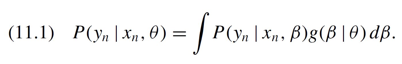
Then, we should integrate the numerator of, say the first parameter, using numerator_B_x1 = MonteCarlo(B_x1_RND * condprobIndiv), which resembles what is contained in equation 11.3 in Train's book.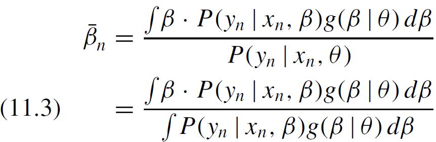
So putting everything together this is what I understand should provide the individual-level parameters:
[Replication code]
Thank you so much for your quick answer. I was, however, trying to understand what to change in BIOGEME in order to implement the individual-level parameters when dealing with panel data, even though theoretically, as you mention it does not make any difference.
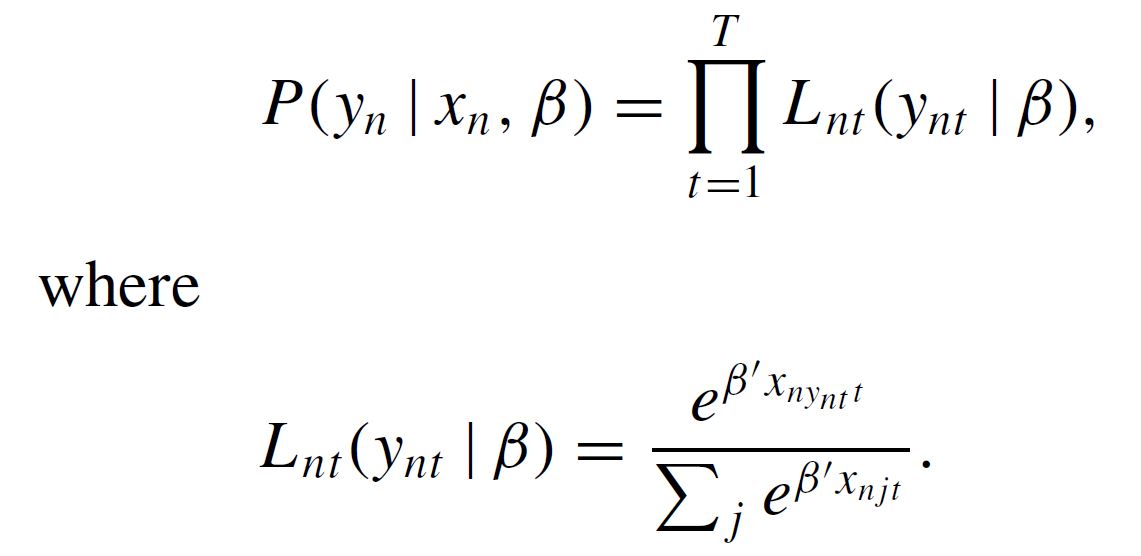
First, what I understand, is that we generate the product of the logit formulas using condprobIndiv = PanelLikelihoodTrajectory(obsprob), that is to say:
Later we will use this expression as the "Denominator" integrating out the beta parameters using denominator = MonteCarlo(condprobIndiv), which performs:
Later we will use this expression as the "Denominator" integrating out the beta parameters using denominator = MonteCarlo(condprobIndiv), which performs:
Then, we should integrate the numerator of, say the first parameter, using numerator_B_x1 = MonteCarlo(B_x1_RND * condprobIndiv), which resembles what is contained in equation 11.3 in Train's book.
So putting everything together this is what I understand should provide the individual-level parameters:
...
obsprob = models.logit(V, av, CHOICE)
condprobIndiv = PanelLikelihoodTrajectory(obsprob)
...####---------------------------------------####
####---- INDIVIDUAL LEVEL PARAMETERS ----####
####---------------------------------------####
# Estimate individual level parameters
numerator_B_x1 = MonteCarlo(B_x1_RND * condprobIndiv)
numerator_B_x2 = MonteCarlo(B_x2_RND * condprobIndiv)
denominator = MonteCarlo(condprobIndiv)
simulate = {'Numerator_B_x1': numerator_B_x1,
'Numerator_B_x2': numerator_B_x2,
'Denominator': denominator}
#integration
biosim = bio.BIOGEME(database,simulate,numberOfDraws=1000)
#Simulation at the estimated values
sim = biosim.simulate(results.data.betaValues)
# Ratio from equation (11.3) Train's Book.
sim['beta_1'] = sim['Numerator_B_x1'] / sim['Denominator']
sim['beta_2'] = sim['Numerator_B_x2'] / sim['Denominator']
However, I am getting the following error, which I haven't been able to solve yet.
File "C:\Users\u0133260\AppData\Local\Continuum\anaconda3\lib\site-packages\spyder_kernels\customize\spydercustomize.py", line 827, in runfile
execfile(filename, namespace)
File "C:\Users\u0133260\AppData\Local\Continuum\anaconda3\lib\site-packages\spyder_kernels\customize\spydercustomize.py", line 110, in execfile
exec(compile(f.read(), filename, 'exec'), namespace)
File "route//file.py", line 137, in <module>
sim = biosim.simulate(results.data.betaValues)
File "C:\Users\u0133260\AppData\Local\Continuum\anaconda3\lib\site-packages\biogeme\biogeme.py", line 773, in simulate
self.database.data)
File "src/cbiogeme.pyx", line 103, in biogeme.cbiogeme.pyBiogeme.simulateFormula
RuntimeError: src/bioExprPanelTrajectory.cc:51: Biogeme exception: Null pointer: data map
Finally, below you might find the entire script for replication purposes.
Thank you a lot again for your time.
Best regards
[Replication code]
# -*- coding: utf-8 -*-
"""
Created on Tue Oct 19 10:24:06 2021
####---- BIOGEME ESTIMATION ----####
biogeme = bio.BIOGEME(database, logprob, numberOfDraws=50)
biogeme.modelName = 'Two_Normally_Distributed_Parameters'
# Estimate the parameters
results = biogeme.estimate()
print(results.getEstimatedParameters())
####---------------------------------------####
####---- INDIVIDUAL LEVEL PARAMETERS ----####
####---------------------------------------####
# Estimate individual level parameters
numerator_B_x1 = MonteCarlo(B_x1_RND * condprobIndiv)
numerator_B_x2 = MonteCarlo(B_x2_RND * condprobIndiv)
denominator = MonteCarlo(condprobIndiv)
simulate = {'Numerator_B_x1': numerator_B_x1,
'Numerator_B_x2': numerator_B_x2,
'Denominator': denominator}
#integration
biosim = bio.BIOGEME(database,simulate,numberOfDraws=1000)
#Simulation at the estimated values
sim = biosim.simulate(results.data.betaValues)
# Ratio from equation (11.3) Train's Book.
sim['beta_1'] = sim['Numerator_B_x1'] / sim['Denominator']
sim['beta_2'] = sim['Numerator_B_x2'] / sim['Denominator']
Bierlaire Michel
Oct 19, 2021, 5:03:43 AM10/19/21
to gutierre...@gmail.com, Bierlaire Michel, Biogeme
Oh, I see.
The simulation does not work if the data is organized as panel data. This feature should be implemented in the next version.
Meanwhile, you can easily reorganize your data such that each individual corresponds to one row, and organize the index t into additional columns.
As an example, here is the swissmetro database organized as such:
On 19 Oct 2021, at 10:26, Álvaro A. Gutiérrez-Vargas <gutierre...@gmail.com> wrote:
Dear Profesor Bierlaire,
Thank you so much for your quick answer. I was, however, trying to understand what to change in BIOGEME in order to implement the individual-level parameters when dealing with panel data, even though theoretically, as you mention it does not make any difference.
First, what I understand, is that we generate the product of the logit formulas using condprobIndiv = PanelLikelihoodTrajectory(obsprob), that is to say:
<f1.JPG>
Later we will use this expression as the "Denominator" integrating out the beta parameters using denominator = MonteCarlo(condprobIndiv), which performs:
<f2.JPG>
Then, we should integrate the numerator of, say the first parameter, using numerator_B_x1 = MonteCarlo(B_x1_RND * condprobIndiv), which resembles what is contained in equation 11.3 in Train's book.
To view this discussion on the web visit https://groups.google.com/d/msgid/biogeme/51900c68-30f2-47c8-aa80-7def8a8b4c08n%40googlegroups.com.
<f1.JPG><f3.JPG><f2.JPG>
Álvaro A. Gutiérrez-Vargas
Oct 19, 2021, 5:57:57 AM10/19/21
to Biogeme
Dear profesor Bierlaire,
thank you again for your quick answer. I've transformed my data (code below in yellow) into the format you mentioned in your previous email, that is to say, my columns do have now the structure "Attribute_Alternative_ChoiceSet". For instance, the column "x1_3_20" stores the value of the attribute "x1" for alternative "3" in the choice set number "20".
However, now I am somewhat confused about how to perform the simulation using such a data structure because it is different from the one I used to estimate the model.
Do you happen to have some sort of example about how to produce posterior distributions for random parameters using said data configuration (i.e., "Attribute_Alternative_ChoiceSet")?
Thank you again for your time.
Best regards,
####---------------------------------------####
####---- INDIVIDUAL LEVEL PARAMETERS ----####
####---------------------------------------####
# First I need to pivot the data in order to create one individual per row and
# multiple choice sets as new columns
df_one_row_per_ind =df.pivot(index='id_ind',
columns='id_choice_situation_of_individual_n',
values=['CHOICE','x1_1','x1_2','x1_3','x2_1','x2_2','x2_3'])
df_one_row_per_ind = df_one_row_per_ind.sort_index(axis=1, level=1)
df_one_row_per_ind.columns = [f'{x}_{y}' for x,y in df_one_row_per_ind.columns]
df_one_row_per_ind = df_one_row_per_ind.reset_index()
'''
id_ind CHOICE_1 x1_1_1 x1_2_1 x1_3_1 x2_1_1 x2_2_1
0 1 3.0 -0.465470 0.150920 -1.083683 0.023137 0.291732
1 2 3.0 0.007468 -0.182140 -0.065210 -0.518345 -0.380828
2 3 3.0 -0.619166 0.663442 1.050588 -1.325250 0.423181
3 4 1.0 0.043973 -0.790810 -0.417802 -0.204473 1.237421
4 5 2.0 -0.240042 0.470926 -0.000197 -0.475226 -0.707226
'''
# Estimate individual level parameters
numerator_B_x1 = MonteCarlo(B_x1_RND * condprobIndiv)
numerator_B_x2 = MonteCarlo(B_x2_RND * condprobIndiv)
denominator = MonteCarlo(condprobIndiv)
simulate = {'Numerator_B_x1': numerator_B_x1,
'Numerator_B_x2': numerator_B_x2,
'Denominator': denominator}
#integration
biosim = bio.BIOGEME(df_one_row_per_ind,simulate,numberOfDraws=1000)
#Simulation at the estimated values
sim = biosim.simulate(results.data.betaValues)
# Ratio from equation (11.3) Train's Book.
sim['beta_1'] = sim['Numerator_B_x1'] / sim['Denominator']
sim['beta_2'] = sim['Numerator_B_x2'] / sim['Denominator']
Bierlaire Michel
Oct 22, 2021, 2:04:36 AM10/22/21
to gutierre...@gmail.com, Bierlaire Michel, Biogeme
You need to explicitly write equation (11.1). First, write the conditional probability as a product on t. This is now possible as the data for all t are available on the same row.
Then you integrate to obtain (11.1).
To view this discussion on the web visit https://groups.google.com/d/msgid/biogeme/58690076-c96a-46b9-8498-7fa1e3c6892bn%40googlegroups.com.
Reply all
Reply to author
Forward
0 new messages