On Robin boundary conditions
395 views
Skip to first unread message

Vyaas Gururajan
Jul 1, 2020, 1:42:49 PM7/1/20
to basilisk-fr
I am trying to understand how exactly the Robin boundary condition (or mixed boundary condition) is applied in the SAG test case bundled with basilisk:
My understanding is that the phrases "dirichlet()" and "neumann()" communicate the needful to the Poisson solver which derives the homogeneous boundary conditions out of these as stated in the manual: http://basilisk.fr/Basilisk%20C#boundary-conditions
In the SAG case, the neumann keyword isn't used; an explicit expression for the ghost cell value is written instead. How does the Poisson solver ultimately handle this?
Thanks,
Vyaas
P.S. I've had a look at the patch by tfullana here but it seems broken for some reason.

"Pierre-Yves Lagrée (PYL)"
Jul 1, 2020, 3:00:33 PM7/1/20
to Vyaas Gururajan, basilisk-fr
Dear Vyaas
A mixed BC, or Robin BC, or even Navier BC is a mix between the value of the flux and the value of the variable at the boundary, here at the bottom (change the sign for the top!)
$$
\frac{\partial c}{\partial y} = bi\; c \;\;\mathrm{on}\;\; y=0
$$
If you discretize it you have a relation between c[] you are looking for and the ghost value c[bottom]
(c[] - c[bottom])/Delta = bi*(c[] + c[bottom])/2.;


hence the BC is:
double bi = 1;
c[bottom] =   c[]*(2. - bi*Delta)/(2. + bi*Delta);
cheers
--
You received this message because you are subscribed to the Google Groups "basilisk-fr" group.
To unsubscribe from this group and stop receiving emails from it, send an email to basilisk-fr...@googlegroups.com.
To view this discussion on the web visit https://groups.google.com/d/msgid/basilisk-fr/f800697d-9257-4c04-8b78-c5d6da267222n%40googlegroups.com.
----> ----> ----> ----> ----> ----> ----> ---->
---> ---> Pierre-Yves Lagrée (PYL) ----> ---->
//////////////////////////////////////////////
Vyaas Gururajan
Jul 1, 2020, 3:24:23 PM7/1/20
to basilisk-fr
Thank you PYL!
The discretization and ghost cell value makes sense to me. What trips me are the following line in the Poisson solver:
for (int b = 0; b < nboundary; b++)
for (scalar s in da)
s.boundary[b] = s.boundary_homogeneous[b];
This is applied to the correction field and the homogeneous boundary condition is inherited from the original scalar 'a'. This is apparently automatically done for dirichlet and neumann conditions. I'm wondering how this line is handled for Robin boundary conditions.
Thanks!
V

j.a.v...@gmail.com
Jul 2, 2020, 3:37:21 AM7/2/20
to basilisk-fr
Hallo Vyaas,
You are right, setting such explicit boundary conditions for a field
that is the solution to a Poisson problem will not always work, because
the homogeneous equivalent is not defined. Meaning that the corrected
fields after a MG cycle may not satisfy boundary conditions.
For the sag.c problem, the solution-centre profile has no gradient at the bottom,
this maybe why it converges. (?although this seems to violate the BC?)
Antoon
Op woensdag 1 juli 2020 om 21:24:23 UTC+2 schreef Vyaas Gururajan:
Vyaas Gururajan
Jul 2, 2020, 10:24:34 AM7/2/20
to j.a.v...@gmail.com, basilisk-fr
Hi Antoon,
> ... setting such explicit boundary conditions
here: http://basilisk.fr/sandbox/tfullana/patch_robinBC and
here: http://basilisk.fr/sandbox/yonghui/smalltest/robin.c
So I rolled up my sleeves and added a Robin (mixed) boundary
condition and its accompanying homogeneous boundary condition
like in the articles above to see if it works. I will summarize
my steps below, show that it works by comparing with an
analytical solution, and then pose a question about how this can
be better done.
1) First, I edit the lines in the qcc.lex source code
(http://basilisk.fr/src/qcc.lex):
> char * cond[2] = {"dirichlet", "neumann"};
is replaced by
> char * cond[3] = {"dirichlet", "neumann", "robin"};
and the iterator five lines below this is appropriately changed
from
> for (i = 0; i < 2; i++)
to
> for (i = 0; i < 3; i++)
After this, I simply recompile qcc.
2) To test if the Robin boundary conditions and their
homogeneous counterparts work, I used an example problem from
Professor Fitzpatrick's notes
(http://farside.ph.utexas.edu/teaching/329/lectures/node66.html)
where he codifies the Robin boundary condition as αu+β∇u=γ where
α, β, and γ are prescribed constants and u is the variable being
solved for. The "robin" boundary conditions are codified for the
lexer as
> double alpha = 0.0e0;
> double beta = 0.0e0;
> double _gamma = 0.0e0;
> @define robin(alpha,beta,_gamma) ((2.*_gamma*Delta/(2.*beta+alpha*Delta)) + ((2.*beta-alpha*Delta)/(2.*beta+alpha*Delta))*val(_s,0,0,0))
> @define robin_homogeneous() (((2.*beta-alpha*Delta)/(2.*beta+alpha*Delta))*val(_s,0,0,0))
I believe the two @define statements ensure the correct boundary
conditions are communicated to the Poisson solver, specifically
the correction fields.
Here is the full code that tests Robin boundary conditions for a
Poisson problem:
> /* This program tests the correctness of the Robin boundary condition: αu+β∇u=γ
> * where α, β, and γ are given constants.*/
>
> double alpha = 0.0e0;
> double beta = 0.0e0;
> double _gamma = 0.0e0;
> @define robin(alpha,beta,_gamma) ((2.*_gamma*Delta/(2.*beta+alpha*Delta)) + ((2.*beta-alpha*Delta)/(2.*beta+alpha*Delta))*val(_s,0,0,0))
> @define robin_homogeneous() (((2.*beta-alpha*Delta)/(2.*beta+alpha*Delta))*val(_s,0,0,0))
>
> #define LEVEL 7
> #include "grid/bitree.h"
> #include "poisson.h"
>
> double alphaL=1.0e0;
> double betaL=-1.0e0;
> double gammaL=1.0e0;
>
> double alphaR=1.0e0;
> double betaR=1.0e0;
> double gammaR=1.0e0;
>
> /* Here is the analaytical solution taken from Professor
> Fitzpatrick's notes
> (http://farside.ph.utexas.edu/teaching/329/lectures/node66.html):*/
>
> double analyticalU(double x){
> double d = alphaL*alphaR+alphaL*betaR-betaL*alphaR;
> double g = (gammaL*(alphaR+betaR)-betaL*(gammaR-(alphaR+betaR)/3.))/d;
> double h = (alphaL*(gammaR-(alphaR+betaR)/3.0e0)-gammaL*alphaR)/d;
> double sqx=x*x;
> double qx=sqx*sqx;
> return(g +h*x +sqx/2.0 -qx/6.0);
> }
>
>
> int main(){
> FILE* output=fopen("output.dat","w");
> size(1.0);
> init_grid(1<<LEVEL);
> scalar u[],rhs[];
>
> foreach(){
> rhs[]=1.0-2.0*sq(x);
> u[]=0.0e0;
> }
>
> alpha=alphaL;
> beta=betaL;
> _gamma=gammaL;
> u[left]=robin(alpha,beta,_gamma);
>
> alpha=alphaR;
> beta=betaR;
> _gamma=gammaR;
> u[right]=robin(alpha,beta,_gamma);
>
> boundary({u});
>
> mgstats mg = poisson(a=u,b=rhs,tolerance=1e-09);
> printf("resbefore: %15.6e resafter: %15.6e minlevel: %d, iters: %d, nrelax: %d\n",
> mg.resb, mg.resa,mg.minlevel,mg.i,mg.nrelax);
>
> foreach(){
> fprintf(output,"%15.6e\t%15.6e\t%15.6e\n",x,u[],analyticalU(x));
> }
>
> free_grid();
> fclose(output);
> exit(0);
> }
One can compile and run the above via "qcc robin.c -lm;./a.out"
(only after the appropriate modifications are made to qcc.lex of
course!).
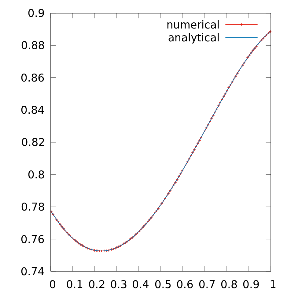
3) See the attached numerical solution compared to the
analytical one. It looks satisfactory to me, especially because
there is a non-zero gradient at both ends (unlike the
aforementioned sag.c test case).
So all this is fine and it looks like for the simplest problems
one can proceed in this fashion.
However, the approach seems messy as it involves entering the
source code and making a modification. I'd much rather use a
user defined subroutine to handle homogeneous boundary
conditions (like the one used in the complex domain Poisson
example here: http://basilisk.fr/src/test/neumann.c ). The thing
is I don't know what the mechanism of passing data is for such a
subroutine and how it ought to be linked correctly to the
scalar. Can someone share a minimal example of how to do this
(if it is even possible)? Is there another way to accomplish the
above without interfering with the source code?
I'll also take this opportunity to congratulate the Basilisk
team on maintaining such a powerful and readily usable code:
there is an invaluable educational emphasis here that I haven't
found much in other numerical code groups and I'm extremely
grateful for that! Thank you Stéphane, Antoon, and everyone
else!
Regards,
Vyaas
> ... setting such explicit boundary conditions
> for a field that is the solution to a Poisson problem will
> not always work, because the homogeneous equivalent is not
> defined. Meaning that the corrected fields after a MG cycle
> may not satisfy boundary conditions.
This is what I suspected, especially after perusing the work
> not always work, because the homogeneous equivalent is not
> defined. Meaning that the corrected fields after a MG cycle
> may not satisfy boundary conditions.
here: http://basilisk.fr/sandbox/tfullana/patch_robinBC and
here: http://basilisk.fr/sandbox/yonghui/smalltest/robin.c
So I rolled up my sleeves and added a Robin (mixed) boundary
condition and its accompanying homogeneous boundary condition
like in the articles above to see if it works. I will summarize
my steps below, show that it works by comparing with an
analytical solution, and then pose a question about how this can
be better done.
1) First, I edit the lines in the qcc.lex source code
(http://basilisk.fr/src/qcc.lex):
> char * cond[2] = {"dirichlet", "neumann"};
is replaced by
> char * cond[3] = {"dirichlet", "neumann", "robin"};
and the iterator five lines below this is appropriately changed
from
> for (i = 0; i < 2; i++)
to
> for (i = 0; i < 3; i++)
After this, I simply recompile qcc.
2) To test if the Robin boundary conditions and their
homogeneous counterparts work, I used an example problem from
Professor Fitzpatrick's notes
(http://farside.ph.utexas.edu/teaching/329/lectures/node66.html)
where he codifies the Robin boundary condition as αu+β∇u=γ where
α, β, and γ are prescribed constants and u is the variable being
solved for. The "robin" boundary conditions are codified for the
lexer as
> double alpha = 0.0e0;
> double beta = 0.0e0;
> double _gamma = 0.0e0;
> @define robin(alpha,beta,_gamma) ((2.*_gamma*Delta/(2.*beta+alpha*Delta)) + ((2.*beta-alpha*Delta)/(2.*beta+alpha*Delta))*val(_s,0,0,0))
> @define robin_homogeneous() (((2.*beta-alpha*Delta)/(2.*beta+alpha*Delta))*val(_s,0,0,0))
I believe the two @define statements ensure the correct boundary
conditions are communicated to the Poisson solver, specifically
the correction fields.
Here is the full code that tests Robin boundary conditions for a
Poisson problem:
> /* This program tests the correctness of the Robin boundary condition: αu+β∇u=γ
> * where α, β, and γ are given constants.*/
>
> double alpha = 0.0e0;
> double beta = 0.0e0;
> double _gamma = 0.0e0;
> @define robin(alpha,beta,_gamma) ((2.*_gamma*Delta/(2.*beta+alpha*Delta)) + ((2.*beta-alpha*Delta)/(2.*beta+alpha*Delta))*val(_s,0,0,0))
> @define robin_homogeneous() (((2.*beta-alpha*Delta)/(2.*beta+alpha*Delta))*val(_s,0,0,0))
>
> #define LEVEL 7
> #include "grid/bitree.h"
> #include "poisson.h"
>
> double alphaL=1.0e0;
> double betaL=-1.0e0;
> double gammaL=1.0e0;
>
> double alphaR=1.0e0;
> double betaR=1.0e0;
> double gammaR=1.0e0;
>
> /* Here is the analaytical solution taken from Professor
> Fitzpatrick's notes
> (http://farside.ph.utexas.edu/teaching/329/lectures/node66.html):*/
>
> double analyticalU(double x){
> double d = alphaL*alphaR+alphaL*betaR-betaL*alphaR;
> double g = (gammaL*(alphaR+betaR)-betaL*(gammaR-(alphaR+betaR)/3.))/d;
> double h = (alphaL*(gammaR-(alphaR+betaR)/3.0e0)-gammaL*alphaR)/d;
> double sqx=x*x;
> double qx=sqx*sqx;
> return(g +h*x +sqx/2.0 -qx/6.0);
> }
>
>
> int main(){
> FILE* output=fopen("output.dat","w");
> size(1.0);
> init_grid(1<<LEVEL);
> scalar u[],rhs[];
>
> foreach(){
> rhs[]=1.0-2.0*sq(x);
> u[]=0.0e0;
> }
>
> alpha=alphaL;
> beta=betaL;
> _gamma=gammaL;
> u[left]=robin(alpha,beta,_gamma);
>
> alpha=alphaR;
> beta=betaR;
> _gamma=gammaR;
> u[right]=robin(alpha,beta,_gamma);
>
> boundary({u});
>
> mgstats mg = poisson(a=u,b=rhs,tolerance=1e-09);
> printf("resbefore: %15.6e resafter: %15.6e minlevel: %d, iters: %d, nrelax: %d\n",
> mg.resb, mg.resa,mg.minlevel,mg.i,mg.nrelax);
>
> foreach(){
> fprintf(output,"%15.6e\t%15.6e\t%15.6e\n",x,u[],analyticalU(x));
> }
>
> free_grid();
> fclose(output);
> exit(0);
> }
One can compile and run the above via "qcc robin.c -lm;./a.out"
(only after the appropriate modifications are made to qcc.lex of
course!).
3) See the attached numerical solution compared to the
analytical one. It looks satisfactory to me, especially because
there is a non-zero gradient at both ends (unlike the
aforementioned sag.c test case).
So all this is fine and it looks like for the simplest problems
one can proceed in this fashion.
However, the approach seems messy as it involves entering the
source code and making a modification. I'd much rather use a
user defined subroutine to handle homogeneous boundary
conditions (like the one used in the complex domain Poisson
example here: http://basilisk.fr/src/test/neumann.c ). The thing
is I don't know what the mechanism of passing data is for such a
subroutine and how it ought to be linked correctly to the
scalar. Can someone share a minimal example of how to do this
(if it is even possible)? Is there another way to accomplish the
above without interfering with the source code?
I'll also take this opportunity to congratulate the Basilisk
team on maintaining such a powerful and readily usable code:
there is an invaluable educational emphasis here that I haven't
found much in other numerical code groups and I'm extremely
grateful for that! Thank you Stéphane, Antoon, and everyone
else!
Regards,
Vyaas

Stephane Popinet
Jul 2, 2020, 10:28:24 AM7/2/20
to basil...@googlegroups.com
Hi Vyaas,
This is very nice. Could you please read:
http://basilisk.fr/src/test/README#running-and-creating-test-cases-and-examples
http://basilisk.fr/src/Contributing
and turn this into a sandbox/patch?
cheers,
Stephane
This is very nice. Could you please read:
http://basilisk.fr/src/test/README#running-and-creating-test-cases-and-examples
http://basilisk.fr/src/Contributing
and turn this into a sandbox/patch?
cheers,
Stephane
Vyaas Gururajan
Jul 2, 2020, 12:47:41 PM7/2/20
to Stephane Popinet, basil...@googlegroups.com
Hi Stephane,
> Could you please read: ... and turn this into a
> sandbox/patch?
I'd love to! It'll give me a chance to learn darcs (I come from
the church of git :p).
I still feel uncomfortable with such a change: I prefer explicit
subroutines over macros. Is there a way to implement subroutines
in this scenario? It'll give the user more control over how data
is being passed around when ghost cells are filled.
Regards,
Vyaas
j.a.v...@gmail.com
Jul 3, 2020, 12:15:39 PM7/3/20
to basilisk-fr
Hallo Vyaas,
> Is there another way to accomplish the
above without interfering with the source code?
above without interfering with the source code?
Yes:
#define robin(a,b,c) ((dirichlet ((c)*Delta/(2*(b) + (a)*Delta))) + ((neumann (0))*((2*(b) - (a)*Delta)/(2*(b) + (a)*Delta) + 1.)))
Enjoy
Antoon
Op donderdag 2 juli 2020 om 18:47:41 UTC+2 schreef Vyaas Gururajan:
Vyaas Gururajan
Jul 3, 2020, 12:37:22 PM7/3/20
to j.a.v...@gmail.com, basilisk-fr
Hi Antoon,
> #define robin(a,b,c) ((dirichlet ((c)*Delta/(2*(b) +
> (a)*Delta))) + ((neumann (0))*((2*(b) - (a)*Delta)/(2*(b) +
> (a)*Delta) + 1.)))
This is dazzlingly brilliant! If I understand correctly, what
you've done is to express the Robin boundary condition as a
superposition of Dirichlet and Neumann conditions. In this way,
the macro is appropriately expanded not only when the ghost
cells are filled for the scalar (via boundary calls), but also
when its homogeneous equivalent is called (via
boundary_homogeneous calls)! Is my interpretation right?
V
> #define robin(a,b,c) ((dirichlet ((c)*Delta/(2*(b) +
> (a)*Delta))) + ((neumann (0))*((2*(b) - (a)*Delta)/(2*(b) +
> (a)*Delta) + 1.)))
you've done is to express the Robin boundary condition as a
superposition of Dirichlet and Neumann conditions. In this way,
the macro is appropriately expanded not only when the ghost
cells are filled for the scalar (via boundary calls), but also
when its homogeneous equivalent is called (via
boundary_homogeneous calls)! Is my interpretation right?
V
j.a.v...@gmail.com
Jul 4, 2020, 5:26:31 AM7/4/20
to basilisk-fr
Hallo Vyaas,
Yes, for a complete narrative and your test see:
Antoon
Op vrijdag 3 juli 2020 om 18:37:22 UTC+2 schreef Vyaas Gururajan:
Vyaas Gururajan
Jul 4, 2020, 10:45:50 AM7/4/20
to j.a.v...@gmail.com, basilisk-fr
Fantastic Antoon!
Apart from the clunky source code manipulations, you have also
addressed another short-coming in my code above:
When the Robin boundary condition is on the left of the
domain, the sign of β (or b in your case) will have to be
changed.
Many thanks!!
V
Apart from the clunky source code manipulations, you have also
addressed another short-coming in my code above:
When the Robin boundary condition is on the left of the
domain, the sign of β (or b in your case) will have to be
changed.
Many thanks!!
V
Reply all
Reply to author
Forward
0 new messages