Recommended solvers for Laplace problem?

[Jonatan Lehtonen]

Hello,

I am trying to solve a 2D Laplace problem with simple Dirichlet boundary conditions (u = 0 on one part of the boundary, u = 1 on another). I mentioned this same problem in my previous post; the only difference is that I want to be able to solve it in a much more general domain than a unit square. The code I'm currently using looks like this: 

mesh = mesh_file_reader(filepath, bc_indices)

domain = FEDomain('domain', mesh)

omega = domain.create_region('Omega', 'all')

gamma0 = domain.create_region('Gamma 0', ' +v '.join('vertices of group {}'.format(n) for n in bc_indices[0]),

 'facet')

gamma1 = domain.create_region('Gamma 1', ' +v '.join('vertices of group {}'.format(n) for n in bc_indices[1]),

 'facet')

field = Field.from_args('fu', nm.float64, 'scalar', omega, approx_order=2)

u = FieldVariable('u', 'unknown', field)

v = FieldVariable('v', 'test', field, primary_var_name='u')

integral = Integral('i', order=2)

term = Term.new('dw_laplace(v, u)', integral, omega, v=v, u=u)

eq = Equation('Laplace equation', term)

eqs = Equations([eq])

ebc0 = EssentialBC('Dirichlet 0', gamma0, {'u.all': 0.0})

ebc1 = EssentialBC('Dirichlet 1', gamma1, {'u.all': 1.0})

pb = Problem('Laplace problem', equations=eqs)

pb.time_update(ebcs=Conditions([ebc0, ebc1]))

vec = pb.solve()

While it's not relevant to the problem at hand, here's two notes about the code above which may seem odd at first glance. Firstly, mesh_file_reader is a custom function which simply reads the necessary data from a .mesh-file generated by gmsh and calls Mesh.from_data() with the appropriate arguments. Secondly, bc_indices contains two tuples of indices which define parts of the boundary; this is just to work around some shortcomings with the gmsh command line interface, but essentially domain.create_region() is called with something like "vertices of group 1 +v vertices of group 2".

Anyway, my goal is to get the highest possible accuracy out of this. The only real limitations here are memory and speed. So basically my question is, given a fixed amount of memory and time, what would be the best choice of solver methods for this problem? Should I just go with the defaults? Also, is there some recommendation for settings such as the mesh order? Memory is my biggest concern; for time consumption something which takes an order of magnitude longer than the default direct solver would still be acceptable.

To clarify, I fully understand that there's no silver bullet that magically solves all my problems, I'm just looking for some pointers about what I should try, as my own experience in FEM solvers is quite limited. Thus far, I've successfully solved the problem with the defaults, and I've tried all the available SciPy iterative solvers to no avail. WIth the iterative solvers, convergence seems much too slow; this is likely because I did not supply a preconditioner, but I'm not entirely sure how that should be done in SfePy, or even what would be an appropriate preconditioner in the first place.

I would greatly appreciate any help with this problem. I can probably work with what I already have, but any performance improvements would certainly be most welcome.

Regards,

Jonatan

PS. An additional somewhat unrelated question. My goal is to solve several hundred of these problems in one execution; each time, the geometry of the mesh changes slightly, but everything else stays the same. Once I start solving a new problem, I don't need the old one anymore, so is there a way of deleting all the SfePy data related to the old problem? That is, I would like to be able to run the code I posted above several hundred times in a row (with different file paths for the mesh_file_reader), without running into memory leak issues. Using the same mesh each time, running the code I posted above results in a peak memory consumption of about 600MB (as reported by the Windows Task Manager) the first time I run it. When I rerun it, the peak memory usage jumps up to 900MB, and after each subsequent repetition the peak memory usage increases by 30MB until eventually I reach 1.3 GB and UMFPACK fails due to running out of memory. As each rerun causes all the variables above to be reassigned, the old ones should be garbage collected, so the only reason I can think of for this happening is that SfePy stores the data somewhere internally. It would be great if there was a way of essentially telling SfePy to start from a clean slate, without having to do trickery like calling SfePy in a temporary subprocess or something like that.

PPS. On the subject of things getting left behind from previous problem solutions, I've noticed that the Probe cache isn't reset when a new problem is solved. This is not unexpected, I'd just like to check whether my workaround for this is correct. What I've done is include the following code after the one I posted above:

from sfepy.discrete.probes import Probe

Probe.cache = pb.domain.get_evaluate_cache(cache=None, share_geometry=True)

Is this the correct way of going about this? The goal is to ensure that subsequent calls to PointsProbe() use the correct cache without needing to explicitly give them a cache object.

[Robert Cimrman]

Hello Jonatan,

On 03/23/2015 12:50 PM, Jonatan Lehtonen wrote:
> Hello,
>
> I am trying to solve a 2D Laplace problem with simple Dirichlet boundary
> conditions (u = 0 on one part of the boundary, u = 1 on another). I
> mentioned this same problem in my previous post

> <https://groups.google.com/forum/#!topic/sfepy-devel/8xgzvEc6Noo>; the only

OK.

> Anyway, my goal is to get the highest possible accuracy out of this. The
> only real limitations here are memory and speed. So basically my question
> is, given a fixed amount of memory and time, what would be the best choice
> of solver methods for this problem? Should I just go with the defaults?
> Also, is there some recommendation for settings such as the mesh order?
> Memory is my biggest concern; for time consumption something which takes an
> order of magnitude longer than the default direct solver would still be
> acceptable.

I recommend installing petsc, petsc4py, and trying something like:

'i10' : ('ls.petsc',
{'method' : 'cg', # ksp_type
'precond' : 'icc', # pc_type
'eps_a' : 1e-12, # abstol
'eps_r' : 1e-12, # rtol
'i_max' : 1000,} # maxits
),

This should be much more memory-friendly than the default direct solver
(umfpack if installed), and also much faster.

BTW. the snippet comes from tests/test_linear_solvers.py - have a look for
other possible solvers. Especially pyamg might be interesting, in case you have
troubles installing petsc with petsc4py.

> To clarify, I fully understand that there's no silver bullet that magically
> solves all my problems, I'm just looking for some pointers about what I
> should try, as my own experience in FEM solvers is quite limited. Thus far,
> I've successfully solved the problem with the defaults, and I've tried all
> the available SciPy iterative solvers to no avail. WIth the iterative
> solvers, convergence seems much too slow; this is likely because I did not
> supply a preconditioner, but I'm not entirely sure how that should be done
> in SfePy, or even what would be an appropriate preconditioner in the first
> place.

You are right, the preconditioning is crucial. The sfepy interface to scipy
solvers lacks that feature (this should be easily fixable - could you add an
enhancement issue?). Luckily, the Laplacian is one of the few problems, where a
silver bullet is sort of known (IIRC) - the conjugate gradients with multigrid
preconditioning (-> try pyamg). Other kinds of preconditioning, such as cg +
icc from petsc proposed above should work very well too.

./run_tests.py tests/test_linear_solvers.py --filter-less

gives on my machine:

... 0.03 [s] (2.428e-12) : i10 ls.petsc cg icc
... 0.05 [s] (3.301e-12) : i20 ls.scipy_iterative cg
... 0.06 [s] (1.046e-12) : i21 ls.scipy_iterative bicgstab
... 0.11 [s] (3.575e-12) : i22 ls.scipy_iterative qmr
... 0.20 [s] (2.634e-12) : i01 ls.pyamg smoothed_aggregation_solver
... 0.29 [s] (3.108e-12) : i00 ls.pyamg ruge_stuben_solver
... 0.33 [s] (4.825e-15) : d00 ls.scipy_direct umfpack
... 1.04 [s] (1.592e-14) : d01 ls.scipy_direct superlu

The test solves the Laplace problem. The times of pyamg are somewhat
misleading, because the test problem is too small, and there is some setup in
amg...

> I would greatly appreciate any help with this problem. I can probably work
> with what I already have, but any performance improvements would certainly
> be most welcome.
>
> Regards,
> Jonatan
>
> PS. An additional somewhat unrelated question. My goal is to solve several
> hundred of these problems in one execution; each time, the geometry of the
> mesh changes slightly, but everything else stays the same. Once I start
> solving a new problem, I don't need the old one anymore, so is there a way
> of deleting all the SfePy data related to the old problem? That is, I would
> like to be able to run the code I posted above several hundred times in a
> row (with different file paths for the mesh_file_reader), without running
> into memory leak issues. Using the same mesh each time, running the code I
> posted above results in a peak memory consumption of about 600MB (as
> reported by the Windows Task Manager) the first time I run it. When I rerun
> it, the peak memory usage jumps up to 900MB, and after each subsequent
> repetition the peak memory usage increases by 30MB until eventually I reach
> 1.3 GB and UMFPACK fails due to running out of memory. As each rerun causes
> all the variables above to be reassigned, the old ones should be garbage
> collected, so the only reason I can think of for this happening is that
> SfePy stores the data somewhere internally. It would be great if there was
> a way of essentially telling SfePy to start from a clean slate, without
> having to do trickery like calling SfePy in a temporary subprocess or
> something like that.

I have found recently as well that the garbage collector is too lazy. When
solving a sequence of problems with different mesh resolutions and
approximation orders, each new Problem instance increased the memory even if
the old one was explicitly deleted. So I did this:

import gc
del pb
gc.collect()

Then the memory increased only for the first two problems (no sure why) and
then stayed bounded. I have used [1] for profiling (mprof run <executable>;
mprof plot).

[1] https://pypi.python.org/pypi/memory_profiler

> PPS. On the subject of things getting left behind from previous problem
> solutions, I've noticed that the Probe cache isn't reset when a new problem
> is solved. This is not unexpected, I'd just like to check whether my
> workaround for this is correct. What I've done is include the following
> code after the one I posted above:
>
> from sfepy.discrete.probes import Probe
> Probe.cache = pb.domain.get_evaluate_cache(cache=None, share_geometry=True)
>
> Is this the correct way of going about this? The goal is to ensure that
> subsequent calls to PointsProbe() use the correct cache without needing to
> explicitly give them a cache object.

Seems OK. BTW. I have just fixed a bug - share_geometry value was ignored by
the probes, so they were always "sharing".

Or you can use:

Probe.cache = pb.domain.get_evaluate_cache(cache=Probe.cache, share_geometry=False)

etc. There is also a new method: Probe.get_evaluate_cache(), which returns the
correct cache, so you could selectively clear, for example, only cache.kdtree,
which depends on coordinates of the mesh, but not cache.iconn, which depends
only on the element connectivity.

Does it help?

r.

[Jonatan Lehtonen]

Hello Robert,

Firstly, thank you for getting back to me so quickly, I really appreciate your help in this.

 

> Anyway, my goal is to get the highest possible accuracy out of this. The
> only real limitations here are memory and speed. So basically my question
> is, given a fixed amount of memory and time, what would be the best choice
> of solver methods for this problem? Should I just go with the defaults?
> Also, is there some recommendation for settings such as the mesh order?
> Memory is my biggest concern; for time consumption something which takes an
> order of magnitude longer than the default direct solver would still be
> acceptable.

I recommend installing petsc, petsc4py, and trying something like:

     'i10' : ('ls.petsc',
              {'method' : 'cg', # ksp_type
               'precond' : 'icc', # pc_type
               'eps_a' : 1e-12, # abstol
               'eps_r' : 1e-12, # rtol
               'i_max' : 1000,} # maxits
     ),

This should be much more memory-friendly than the default direct solver
(umfpack if installed), and also much faster.

BTW. the snippet comes from tests/test_linear_solvers.py - have a look for
other possible solvers. Especially pyamg might be interesting, in case you have
troubles installing petsc with petsc4py.

I assume that this is equivalent to passing ls=PETScKrylovSolver({'method': 'cg', 'precond': 'icc', 'eps_a': 1e-14, 'eps_r': 1e-14, 'i_max': 1000} to the Problem-instance. I tried this on my machine, both with the rectangle2D.mesh from my earlier post and with the mesh I will actually be using (which is closer in shape to one half of an annulus -- still, not a particularly complex geometry). I refined the rectangle mesh twice, so it had 53761 nodes and 106720 triangle elements (the other mesh incidentally has almost exactly the same amount of elements and nodes). I also tried PyAMG by passing ls=PyAMGSolver({'method': 'smoothed_aggregation_solver', 'accel': 'cg', 'eps_r': 1e-14, 'i_max': 1000}) to Problem.

Anyway, with the rectangle (or rather, unit square) mesh, I got the following results for SciPy direct, PETSc and PyAMG respectively:

PETSc:

sfepy:   cg(icc) convergence: -3 (DIVERGED_MAX_IT)

sfepy:     rezidual:    0.13 [s]

sfepy:        solve:   16.81 [s]

sfepy:       matrix:    0.22 [s]

sfepy:   nls: iter: 1, residual: 2.101475e-12 (rel: 5.649462e-14)

PyAMG:

sfepy:   nls: iter: 0, residual: 3.719779e+01 (rel: 1.000000e+00)

sfepy:     rezidual:    0.14 [s]

sfepy:        solve:    4.68 [s]

sfepy:       matrix:    0.24 [s]

sfepy:   nls: iter: 1, residual: 3.051773e-13 (rel: 8.204179e-15)

SciPy direct:

sfepy:   nls: iter: 0, residual: 3.719779e+01 (rel: 1.000000e+00)

sfepy:     rezidual:    0.14 [s]

sfepy:        solve:    8.40 [s]

sfepy:       matrix:    0.23 [s]

sfepy:   nls: iter: 1, residual: 1.903553e-13 (rel: 5.117383e-15)

So even for the unit square, PETSc failed to converge. Granted, it did reach a residual of under 1e-11, but I would have expected full convergence with 1000 iterations on a unit square Laplace problem. PyAMG does beat the SciPy direct solver by a factor of 2. I haven't figured out a good way to test the memory usage yet (as it seems most tools are unable to measure peak memory usage, which is what I'm most concerned about). Anyway, the same tests on the other mesh yielded the following:

PETSc:

sfepy:   nls: iter: 0, residual: 2.460459e+01 (rel: 1.000000e+00)

sfepy:   cg(icc) convergence: -3 (DIVERGED_MAX_IT)

sfepy:     rezidual:    0.14 [s]

sfepy:        solve:   21.61 [s]

sfepy:       matrix:    0.26 [s]

sfepy:   warning: linear system solution precision is lower

sfepy:   then the value set in solver options! (err = 5.747744e-08 < 1.000000e-10)

sfepy:   nls: iter: 1, residual: 5.747744e-08 (rel: 2.336046e-09)

PyAMG:

sfepy:   nls: iter: 0, residual: 2.460459e+01 (rel: 1.000000e+00)

sfepy:     rezidual:    0.15 [s]

sfepy:        solve:    5.59 [s]

sfepy:       matrix:    0.27 [s]

sfepy:   nls: iter: 1, residual: 3.092312e-13 (rel: 1.256803e-14)

SciPy direct:

sfepy:   nls: iter: 0, residual: 2.460459e+01 (rel: 1.000000e+00)

sfepy:     rezidual:    0.15 [s]

sfepy:        solve:    6.94 [s]

sfepy:       matrix:    0.26 [s]

sfepy:   nls: iter: 1, residual: 1.918560e-13 (rel: 7.797571e-15)

As you can see, PETSc performance is even worse now, and PyAMG has lost most of its speed benefit (although I still expect the memory benefit to be significant). Are there some other PyAMG-solvers which I may have overlooked? The SfePy-documentation says that smoothed_aggregation_solver is the default, presumably with good reason. I did also try the ruge_stuben_solver, but that one took 3-4 times as long as smoothed_aggregation_solver to converge.

Now, based on these results, I'll probably go with PyAMG moving forward. The reason I've posted them here though is that the timings and accuracies above don't seem to match your predictions about how well PETSc and PyAMG should fare. I can't help but wonder if there might be some subtle problems with my installations of these solvers, even though my results on test_linear_solvers.py are similar to yours; see below.

 

> To clarify, I fully understand that there's no silver bullet that magically
> solves all my problems, I'm just looking for some pointers about what I
> should try, as my own experience in FEM solvers is quite limited. Thus far,
> I've successfully solved the problem with the defaults, and I've tried all
> the available SciPy iterative solvers to no avail. WIth the iterative
> solvers, convergence seems much too slow; this is likely because I did not
> supply a preconditioner, but I'm not entirely sure how that should be done
> in SfePy, or even what would be an appropriate preconditioner in the first
> place.

You are right, the preconditioning is crucial. The sfepy interface to scipy
solvers lacks that feature (this should be easily fixable - could you add an
enhancement issue?).

Sorry, I'm not entirely sure what you mean by the interface lacking this feature; the documentation at http://sfepy.org/doc-devel/src/sfepy/solvers/ls.html#sfepy.solvers.ls.ScipyIterative does allow for a precond-parameter, but maybe that just doesn't do enough? I would gladly add an issue about this if that helps you, but I just don't know what I should write in it.

 

Luckily, the Laplacian is one of the few problems, where a
silver bullet is sort of known (IIRC) - the conjugate gradients with multigrid
preconditioning (-> try pyamg). Other kinds of preconditioning, such as cg +
icc from petsc proposed above should work very well too.

./run_tests.py tests/test_linear_solvers.py --filter-less

gives on my machine:

...   0.03 [s] (2.428e-12) : i10 ls.petsc cg icc
...   0.05 [s] (3.301e-12) : i20 ls.scipy_iterative cg
...   0.06 [s] (1.046e-12) : i21 ls.scipy_iterative bicgstab
...   0.11 [s] (3.575e-12) : i22 ls.scipy_iterative qmr
...   0.20 [s] (2.634e-12) : i01 ls.pyamg smoothed_aggregation_solver
...   0.29 [s] (3.108e-12) : i00 ls.pyamg ruge_stuben_solver
...   0.33 [s] (4.825e-15) : d00 ls.scipy_direct umfpack
...   1.04 [s] (1.592e-14) : d01 ls.scipy_direct superlu

The test solves the Laplace problem. The times of pyamg are somewhat
misleading, because the test problem is too small, and there is some setup in
amg...

I ran the same test on my machine. My test script is possibly an older version since it doesn't distinguish between scipy_direct umfpack and scipy_direct superlu; the test is the one that's part of SfePy 2015.1, as I'm not yet using a development version. Here are my results:

...   0.05 [s] (2.428e-12) : i10 ls.petsc cg icc

...   0.09 [s] (3.300e-12) : i20 ls.scipy_iterative cg

...   0.13 [s] (3.281e-12) : i21 ls.scipy_iterative bicgstab

...   0.28 [s] (3.012e-12) : i22 ls.scipy_iterative qmr

...   0.75 [s] (3.108e-12) : i00 ls.pyamg ruge_stuben_solver

...   1.14 [s] (2.634e-12) : i01 ls.pyamg smoothed_aggregation_solver

...   1.96 [s] (4.801e-15) : d00 ls.scipy_direct

There is only one test for scipy_direct (which is with 'd00': ('ls.scipy_direct', {'warn' : True, })). I assume this defaults to UMFPACK, as 'd01' is commented out in my version of the test and that one explicitly names the method as 'superlu'.

So it seems that all the solvers are working correctly; however, as I demonstrated earlier, any speed benefit they have over SciPy direct seem to vanish with a denser 2D mesh. Again, I'm happy to just accept the improvement in memory usage, I'm just wondering if maybe I've made some mistake or if there might be something wrong with my PETSc/PyAMG installation.

Unfortunately, this does not solve my memory problems. It does help to some extent, but the increasing trend in memory usage is still present. In order to test the memory leak, I wrote the following code:

import gc

import psutil

import os

from sfepy.base.base import output

output.set_output(quiet=True)

def get_mem_usage():

    process = psutil.Process(os.getpid())

    mem = process.get_memory_info()[0] / float(2 ** 10)

    print("{} KB in use.".format(int(mem)))

def mem_tester(n, refinement_level=0):

    from sfepy.discrete.fem.utils import refine_mesh

    from sfepy.discrete.fem import FEDomain

    from sfepy.discrete.fem.mesh import Mesh

    for i in xrange(0, n):

        mesh = Mesh.from_file(refine_mesh('rectangle2D.mesh', refinement_level))

        domain = FEDomain('domain', mesh)

        del mesh, domain

        gc.collect()

        get_mem_usage()

def mem_tester_complete(n, refinement_level=0):

    from sfepy.discrete.fem.utils import refine_mesh

    from sfepy.discrete import (FieldVariable, Integral, Equation, Equations, Problem)

    from sfepy.discrete.fem import (FEDomain, Field)

    from sfepy.terms import Term

    from sfepy.discrete.conditions import Conditions, EssentialBC

    from sfepy.discrete.fem.mesh import Mesh

    for i in xrange(0, n):

        mesh = Mesh.from_file(refine_mesh('rectangle2D.mesh', refinement_level))

        domain = FEDomain('domain', mesh)

        omega = domain.create_region('Omega', 'all')

        gamma0 = domain.create_region('Gamma 0', 'vertices in (x < 0.00001)', 'facet')

        gamma1 = domain.create_region('Gamma 1', 'vertices in (x > 0.99999)', 'facet')

        field = Field.from_args('fu', np.float64, 'scalar', omega, approx_order=2)

        u = FieldVariable('u', 'unknown', field)

        v = FieldVariable('v', 'test', field, primary_var_name='u')

        integral = Integral('i', order=2)

        term = Term.new('dw_laplace(v, u)', integral, omega, v=v, u=u)

        eq = Equation('Laplace equation', term)

        eqs = Equations([eq])

        ebc0 = EssentialBC('Dirichlet 0', gamma0, {'u.all': 0.0})

        ebc1 = EssentialBC('Dirichlet 1', gamma1, {'u.all': 1.0})

        pb = Problem('Laplace problem', equations=eqs)

        pb.time_update(ebcs=Conditions([ebc0, ebc1]))

        vec = pb.solve()

        gc.collect()

        get_mem_usage()

The mesh, "rectangle2D.mesh", is the same one I used before (and can be found in the previous thread I started about probing and nans). Both mem_tester and mem_tester_complete seem to leak roughly the same amount of memory (the latter does this a bit more sporadically due to the lack of explicit del-calls); on my machine, refinement_level=0 results in 1MB leaked per iteration, and this increases to 7MB and 35MB with refinement levels 1 and 2, respectively. It looks like this will become a significant problem for me, as about 10-20 iterations will leak more memory than it takes to solve the problem, and I'm looking at potentially solving over a thousand problems in one execution.

If you run the code above and don't see a memory leak, I suggest you run at least 100 iterations or so. When I ran the code, I noticed that sometimes the memory usage stayed constant for the first 20 iterations or so.

I understand that something like this can be very tough to solve (unless of course it's me who has made some subtle mistake here); in fact, this memory leak is mild compared to the new FEM package in Mathematica 10, which is what I previously used. Of course I can look into ways of containing the memory leak by making a new thread/process every few iterations or something like that. This is precisely what I ended up doing in Mathematica, although I'm not entirely sure how this should be done in Python. Also, I'm happy to add an issue about this if you'd like.

 

> PPS. On the subject of things getting left behind from previous problem
> solutions, I've noticed that the Probe cache isn't reset when a new problem
> is solved. This is not unexpected, I'd just like to check whether my
> workaround for this is correct. What I've done is include the following
> code after the one I posted above:
>
> from sfepy.discrete.probes import Probe
> Probe.cache = pb.domain.get_evaluate_cache(cache=None, share_geometry=True)
 >
> Is this the correct way of going about this? The goal is to ensure that
> subsequent calls to PointsProbe() use the correct cache without needing to
> explicitly give them a cache object.

Seems OK. BTW. I have just fixed a bug - share_geometry value was ignored by
the probes, so they were always "sharing".

Or you can use:

Probe.cache = pb.domain.get_evaluate_cache(cache=Probe.cache, share_geometry=False)

etc. There is also a new method: Probe.get_evaluate_cache(), which returns the
correct cache, so you could selectively clear, for example, only cache.kdtree,
which depends on coordinates of the mesh, but not cache.iconn, which depends
only on the element connectivity.

Does it help?

r.

I haven't had time to look into your alternate suggestions yet, but just the knowledge that my own code looks alright is good enough for me (and that code seems to work correctly).

Thank you again for all your help!

Regards,

Jonatan

[Robert Cimrman]

Yes, that should be it.

> rectangle2D.mesh from my earlier post and with the mesh I will actually be
> using (which is closer in shape to one half of an annulus -- still, not a
> particularly complex geometry). I refined the rectangle mesh twice, so it
> had 53761 nodes and 106720 triangle elements (the other mesh incidentally
> has almost exactly the same amount of elements and nodes). I also tried
> PyAMG by passing ls=PyAMGSolver({'method': 'smoothed_aggregation_solver',
> 'accel': 'cg', 'eps_r': 1e-14, 'i_max': 1000}) to Problem.

The number of nodes is still rather small.

Do you use some special material properties (like lots of jumps in a coefficient)?

> Now, based on these results, I'll probably go with PyAMG moving forward.
> The reason I've posted them here though is that the timings and accuracies
> above don't seem to match your predictions about how well PETSc and PyAMG
> should fare. I can't help but wonder if there might be some subtle problems
> with my installations of these solvers, even though my results on
> test_linear_solvers.py are similar to yours; see below.

Maybe send me your test script, for verification of the timings?

My bad, I overlooked that one. No work then :)

You can use it by importing scipy.sparse.linalg as spl and creating a
spl.LinearOperator with a proper matvec() - matvec(x) would contain e.g. and
incomplete Cholesky action on a vector x. I do not know, where to get that
readily, though =:).

This seems quite reasonable.

> There is only one test for scipy_direct (which is with 'd00':
> ('ls.scipy_direct', {'warn' : True, })). I assume this defaults to UMFPACK,
> as 'd01' is commented out in my version of the test and that one explicitly
> names the method as 'superlu'.

Yes, this was a recent addition.

> So it seems that all the solvers are working correctly; however, as I
> demonstrated earlier, any speed benefit they have over SciPy direct seem to
> vanish with a denser 2D mesh. Again, I'm happy to just accept the
> improvement in memory usage, I'm just wondering if maybe I've made some
> mistake or if there might be something wrong with my PETSc/PyAMG
> installation.

Let me try it with your script then.

Yes, please, add a new issue. I can reproduce the leak with your script.

BTW. I have left only the domain creation in the loop and it still leaks - I
suspect something wrong in cmesh.pyx. When I comment out the CMesh creation in
FEDomain.__init__(), the leak seems to disappear.

r.

[Jonatan Lehtonen]

Hello Robert,

I have attached the mesh file and the script you asked for, which reproduces the first set of timings I gave in my previous post. The problem is essentially the same one I used in my memory test example. There is no material coefficient, I am just solving the equation Laplacian(u) = 0 with simple Dirichlet boundary conditions u = 0 and u = 1.

Also, I added an issue for the memory leak. :)

Regards,

Jonatan

PS. In case you're interested, the reason I'm solving this problem is to obtain a conformal mapping from an (essentially arbitrary) 2D region to a rectangle, using the method outlined in this article. So the basic idea is to solve two Laplace problems with different boundary conditions and combine the solution to obtain a conformal mapping. Of course, in this example I've used, the solution is trivial since the mesh itself is a unit square. =) 

Speaking of which, the above results in two uncoupled Laplace equations to be solved. Do you think there would be problems with solving these both in one go (that is, adding both equations to the same Problem-instance)? I've tried this, and Scipy direct warns about the system matrix being close to singular, but it seems to solve the problem just fine (and faster than solving two separate problems, with lower overall memory consumption). I'm just wondering, is this sort of approach ill-advised or even potentially unstable?

[Robert Cimrman]

On 03/24/2015 07:37 PM, Jonatan Lehtonen wrote:
> Hello Robert,
>
> I have attached the mesh file and the script you asked for, which
> reproduces the first set of timings I gave in my previous post. The problem
> is essentially the same one I used in my memory test example. There is no
> material coefficient, I am just solving the equation Laplacian(u) = 0 with
> simple Dirichlet boundary conditions u = 0 and u = 1.

I have played with it a bit and found, that the gamg (Geometric algebraic
multigrid (AMG), see [1]) preconditioner from petsc works quite well.

[1] http://www.mcs.anl.gov/petsc/documentation/linearsolvertable.html

I have also modified a bit the script:
- the domain is refined in memory, without wasting time on saving and loading
the text files.
- added context managers for memory_profiler:
- to be run with: mprof run --python laplace.py
- view the memory usage: mprof plot

These are my observations, opinions (IMHO, AFAIK, IIRC etc.):
- in 2D, a good direct solver is hard to beat.
- P1 approximation, where the matrix is more sparse, are better for iterative
solvers than P2 etc.
- staying with pyamg seems a good strategy overall, but petsc cg+gamg behaves
similarly - there some memory might be wasted do to copying data from
numpy.scipy to petsc.

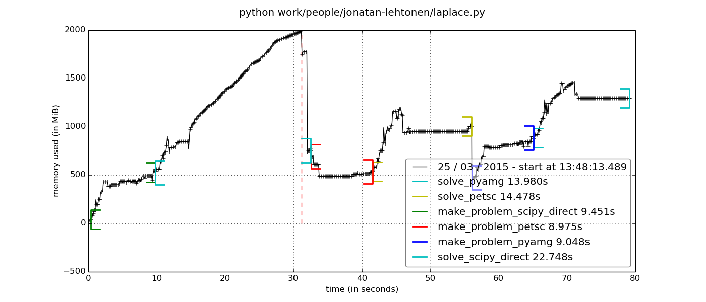
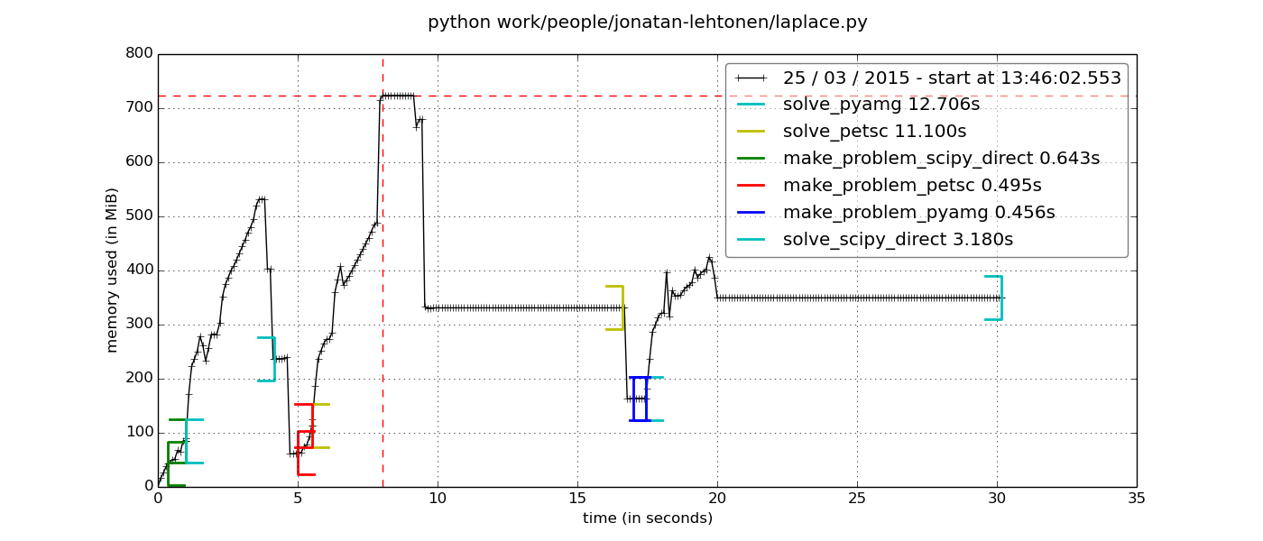
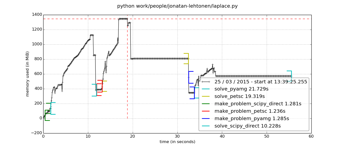
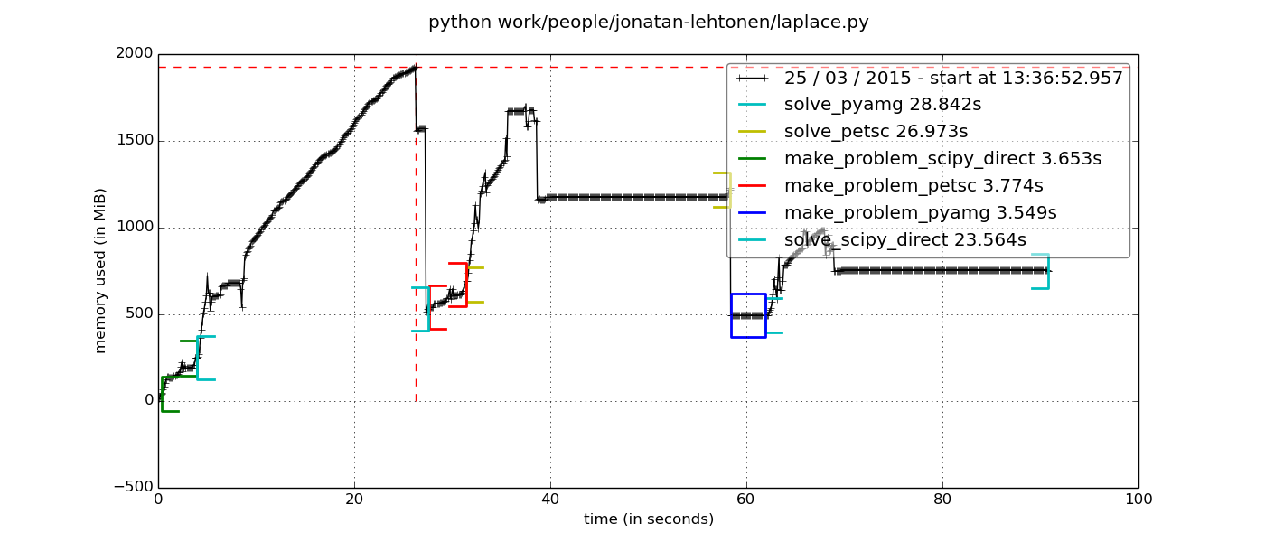
The attached plots show the memory usage and time spent, with names
r<refinement>_p<field_order>.png

> Also, I added an issue for the memory leak. :)

Closed already :)

> Regards,
> Jonatan
>
> PS. In case you're interested, the reason I'm solving this problem is to
> obtain a conformal mapping from an (essentially arbitrary) 2D region to a
> rectangle, using the method outlined in this article

> <http://math.aalto.fi/~vquach/work/publication/hqr-cam-final.pdf>. So the

> basic idea is to solve two Laplace problems with different boundary
> conditions and combine the solution to obtain a conformal mapping. Of
> course, in this example I've used, the solution is trivial since the mesh
> itself is a unit square. =)

Interesting! I will look at the article. What are the applications?

> Speaking of which, the above results in two uncoupled Laplace equations to
> be solved. Do you think there would be problems with solving these both in
> one go (that is, adding both equations to the same Problem-instance)? I've
> tried this, and Scipy direct warns about the system matrix being close to
> singular, but it seems to solve the problem just fine (and faster than
> solving two separate problems, with lower overall memory consumption). I'm
> just wondering, is this sort of approach ill-advised or even potentially
> unstable?
>

It should be ok. I just wonder, why the solver complains about a singular
matrix, when each of the problems has proper Dirichelt BCs... As a side note
see [2].

r.

[2]
http://sfepy.org/doc-devel/examples/thermo_elasticity/thermo_elasticity_ess.html

[Jonatan Lehtonen]

On Wednesday, March 25, 2015 at 2:52:11 PM UTC+2, Robert Cimrman wrote:

On 03/24/2015 07:37 PM, Jonatan Lehtonen wrote:
> Hello Robert,
>
> I have attached the mesh file and the script you asked for, which
> reproduces the first set of timings I gave in my previous post. The problem
> is essentially the same one I used in my memory test example. There is no
> material coefficient, I am just solving the equation Laplacian(u) = 0 with
> simple Dirichlet boundary conditions u = 0 and u = 1.

I have played with it a bit and found, that the gamg (Geometric algebraic
multigrid (AMG), see [1]) preconditioner from petsc works quite well.

[1] http://www.mcs.anl.gov/petsc/documentation/linearsolvertable.html

I have also modified a bit the script:
- the domain is refined in memory, without wasting time on saving and loading
the text files.
- added context managers for memory_profiler:
   - to be run with: mprof run --python laplace.py
   - view the memory usage: mprof plot

I never knew about the plot option of memory_profiler. That's a really cool feature, since only reporting the memory usage line-by-line hides the thing we're really interested in (which is the internal memory usage of pb.solve()).

 

These are my observations, opinions (IMHO, AFAIK, IIRC etc.):
- in 2D, a good direct solver is hard to beat.
- P1 approximation, where the matrix is more sparse, are better for iterative
solvers than P2 etc.
- staying with pyamg seems a good strategy overall, but petsc cg+gamg behaves
similarly - there some memory might be wasted do to copying data from
numpy.scipy to petsc.

The attached plots show the memory usage and time spent, with names
r<refinement>_p<field_order>.png

These plots are very interesting, and the gamg preconditioner looks like a great find! I'll have to play around with the problem some more to figure out which method/order/refinement I'll settle on. Once again, thank you so much for your help! =)

 

> Also, I added an issue for the memory leak. :)

Closed already :)

You do work quickly. =)

 

 

> Regards,
> Jonatan
>
> PS. In case you're interested, the reason I'm solving this problem is to
> obtain a conformal mapping from an (essentially arbitrary) 2D region to a
> rectangle, using the method outlined in this article
> <http://math.aalto.fi/~vquach/work/publication/hqr-cam-final.pdf>. So the
> basic idea is to solve two Laplace problems with different boundary
> conditions and combine the solution to obtain a conformal mapping. Of
> course, in this example I've used, the solution is trivial since the mesh
> itself is a unit square. =)

Interesting! I will look at the article. What are the applications? 

In this particular case, it's related to my master's thesis (a lengthy read, but I'll give the link anyway), where the goal was to e.g. compute stresses in an elastic body as a function of its shape. So if the shape depends on some parameters, then the goal is to compute the stress at some point as a function of those parameters. The problem there is that since the geometry changes, we can't just measure stresses at the same point regardless of the geometry, since the point might land outside the elastic body for some values of the parameters. So, we used conformal mappings to map the solution in any given elastic body to a reference object; then we can pick a measurement point in the reference object instead, without needing to worry about the changing geometry.

Strictly speaking, in this application we don't really care about the fact that the mapping is conformal; in fact, the way we use it, the resulting mapping isn't quite conformal (although it's close). But in other applications, the conformality is actually relevant, and typically allows you to convert a difficult problem into a much simpler one. The article I linked refers to some such applications.

 

> Speaking of which, the above results in two uncoupled Laplace equations to
> be solved. Do you think there would be problems with solving these both in
> one go (that is, adding both equations to the same Problem-instance)? I've
> tried this, and Scipy direct warns about the system matrix being close to
> singular, but it seems to solve the problem just fine (and faster than
> solving two separate problems, with lower overall memory consumption). I'm
> just wondering, is this sort of approach ill-advised or even potentially
> unstable?
>

It should be ok. I just wonder, why the solver complains about a singular
matrix, when each of the problems has proper Dirichelt BCs... As a side note
see [2].

r.

[2]
http://sfepy.org/doc-devel/examples/thermo_elasticity/thermo_elasticity_ess.html

It turned out to be a case of "problem exists between keyboard and chair". Your mention of the BCs prompted me to recheck my code, and indeed, I had accidentally applied the boundary conditions of both Laplace problems to the variable of the first one. Fixing that removed any warning about singularity. =)

By the way, one thing I wasn't entirely sure of when writing this "combined" solver was which objects can be shared between the two equations. The code I've used (excluding mesh generation) is below, and conj (short for conjugate) stands for the second of the two problems. Am I right in assuming that domain, omega, field and integral can be shared by both equations, and everything else needs to be separated, like I've done below? I'm fairly sure the rest of this is correct, but not quite certain if the field can be shared.

domain = FEDomain('domain', mesh)

omega = domain.create_region('Omega', 'all')

gamma0 = domain.create_region('Gamma 0', ' +v '.join('vertices of group {}'.format(n) for n in bc_indices[0][0]), 'facet')

gamma1 = domain.create_region('Gamma 1', ' +v '.join('vertices of group {}'.format(n) for n in bc_indices[0][1]), 'facet')

gamma0_conj = domain.create_region('Gamma 0 conj', ' +v '.join('vertices of group {}'.format(n) for n in bc_indices[1][0]), 'facet')

gamma1_conj = domain.create_region('Gamma 1 conj', ' +v '.join('vertices of group {}'.format(n) for n in bc_indices[1][1]), 'facet')

field = Field.from_args('fu', np.float64, 'scalar', omega, approx_order=2)

u = FieldVariable('u', 'unknown', field)

v = FieldVariable('v', 'test', field, primary_var_name='u')

u_conj = FieldVariable('u_conj', 'unknown', field)

v_conj = FieldVariable('v_conj', 'test', field, primary_var_name='u_conj')

integral = Integral('i', order=2)

term = Term.new('dw_laplace(v, u)', integral, omega, v=v, u=u)

term_conj = Term.new('dw_laplace(v_conj, u_conj)', integral, omega, v_conj=v_conj, u_conj=u_conj)

eq = Equation('Laplace equation', term)

eq_conj = Equation('Laplace equation conj', term_conj)

eqs = Equations([eq, eq_conj])

ebc0 = EssentialBC('Dirichlet 0', gamma0, {'u.all': 0.0})

ebc1 = EssentialBC('Dirichlet 1', gamma1, {'u.all': 1.0})

ebc0_conj = EssentialBC('Dirichlet 0 conj', gamma0_conj, {'u_conj.all': 0.0})

ebc1_conj = EssentialBC('Dirichlet 1 conj', gamma1_conj, {'u_conj.all': 1.0})

pb = Problem('Laplace problem', equations=eqs, nls=nls, ls=ls)

pb.time_update(ebcs=Conditions([ebc0, ebc1, ebc0_conj, ebc1_conj]))

vec = pb.solve()

[Robert Cimrman]

On 03/25/2015 03:09 PM, Jonatan Lehtonen wrote:
> On Wednesday, March 25, 2015 at 2:52:11 PM UTC+2, Robert Cimrman wrote:
>> I have also modified a bit the script:
>> - the domain is refined in memory, without wasting time on saving and
>> loading
>> the text files.
>> - added context managers for memory_profiler:
>> - to be run with: mprof run --python laplace.py
>> - view the memory usage: mprof plot
>>
>
> I never knew about the plot option of memory_profiler. That's a really cool
> feature, since only reporting the memory usage line-by-line hides the thing
> we're really interested in (which is the internal memory usage of
> pb.solve()).

Yes, the time-stamping mode is really useful - you can set also the sampling
frequency.

>> The attached plots show the memory usage and time spent, with names
>> r<refinement>_p<field_order>.png
>
> These plots are very interesting, and the gamg preconditioner looks like a
> great find! I'll have to play around with the problem some more to figure
> out which method/order/refinement I'll settle on. Once again, thank you so
> much for your help! =)

Hth, those are interesting findings. Thanks for debugging!

> In this particular case, it's related to my master's thesis

> <http://urn.fi/URN:NBN:fi:aalto-201503062021> (a lengthy read, but I'll

> give the link anyway), where the goal was to e.g. compute stresses in an
> elastic body as a function of its shape. So if the shape depends on some
> parameters, then the goal is to compute the stress at some point as a
> function of those parameters. The problem there is that since the geometry
> changes, we can't just measure stresses at the same point regardless of the
> geometry, since the point might land outside the elastic body for some
> values of the parameters. So, we used conformal mappings to map the
> solution in any given elastic body to a reference object; then we can pick
> a measurement point in the reference object instead, without needing to
> worry about the changing geometry.
>
> Strictly speaking, in this application we don't really care about the fact
> that the mapping is conformal; in fact, the way we use it, the resulting
> mapping isn't quite conformal (although it's close). But in other
> applications, the conformality is actually relevant, and typically allows
> you to convert a difficult problem into a much simpler one. The article I
> linked refers to some such applications.

Thanks for explanation, it sounds really interesting and useful.

>> It should be ok. I just wonder, why the solver complains about a singular
>> matrix, when each of the problems has proper Dirichelt BCs... As a side
>> note
>> see [2].
>>
>> r.
>>
>> [2]
>>
>> http://sfepy.org/doc-devel/examples/thermo_elasticity/thermo_elasticity_ess.html

>> <http://www.google.com/url?q=http%3A%2F%2Fsfepy.org%2Fdoc-devel%2Fexamples%2Fthermo_elasticity%2Fthermo_elasticity_ess.html&sa=D&sntz=1&usg=AFQjCNEYnCYCzn7O72031QeorR_U3JJVvg>

>>
>
> It turned out to be a case of "problem exists between keyboard and chair".
> Your mention of the BCs prompted me to recheck my code, and indeed, I had
> accidentally applied the boundary conditions of both Laplace problems to
> the variable of the first one. Fixing that removed any warning about
> singularity. =)

So this one was easy :)

> By the way, one thing I wasn't entirely sure of when writing this
> "combined" solver was which objects can be shared between the two
> equations. The code I've used (excluding mesh generation) is below, and
> conj (short for conjugate) stands for the second of the two problems. Am I
> right in assuming that domain, omega, field and integral can be shared by
> both equations, and everything else needs to be separated, like I've done
> below? I'm fairly sure the rest of this is correct, but not quite certain
> if the field can be shared.

You can share a field for as many variables as you need. The field only defines
the approximation (the FE basis), but the actual degrees of freedom to solve
for are determined by the variables.

So yes, everything can be shared (domain, regions, materials, solvers...).

r.

[Jonatan Lehtonen]

> By the way, one thing I wasn't entirely sure of when writing this
> "combined" solver was which objects can be shared between the two
> equations. The code I've used (excluding mesh generation) is below, and
> conj (short for conjugate) stands for the second of the two problems. Am I
> right in assuming that domain, omega, field and integral can be shared by
> both equations, and everything else needs to be separated, like I've done
> below? I'm fairly sure the rest of this is correct, but not quite certain
> if the field can be shared.

You can share a field for as many variables as you need. The field only defines
the approximation (the FE basis), but the actual degrees of freedom to solve
for are determined by the variables.

So yes, everything can be shared (domain, regions, materials, solvers...).

r.

Thank you for confirming that. I played around with this a bit, and it seems these can even be shared by different Problem-instances. However, I did find one exception: the PETSc-solver cannot be reused if the size of the system matrix is different in the two problems. This naturally happens if you use a different mesh for the two problems, but it also occurs if your Dirichlet boundary conditions do not include the exact same number of vertices. I've attached a script which reproduces the problem. I assume this is a bug, just wanted to run it by you before posting an issue about it. Using either of the commented-out lines for ls works just fine (that is, SciPy Direct or PyAMG), but using PETSc produces the following output:

sfepy: reading mesh [line2, tri3, quad4, tetra4, hexa8] (rectangle2D.mesh)...

sfepy: ...done in 0.04 s

sfepy: updating variables...

sfepy: ...done

sfepy: setting up dof connectivities...

sfepy: ...done in 0.00 s

sfepy: matrix shape: (13339, 13339)

sfepy: assembling matrix graph...

sfepy: ...done in 0.01 s

sfepy: matrix structural nonzeros: 151257 (8.50e-04% fill)

sfepy: updating materials...

sfepy: ...done in 0.00 s

sfepy: nls: iter: 0, residual: 1.856814e+01 (rel: 1.000000e+00)

sfepy: cg(gamg) convergence: 2 (CONVERGED_RTOL)

sfepy:   rezidual:    0.01 [s]

sfepy:      solve:    0.25 [s]

sfepy:     matrix:    0.02 [s]

sfepy: nls: iter: 1, residual: 8.178809e-14 (rel: 4.404754e-15)

sfepy: updating variables...

sfepy: ...done

sfepy: setting up dof connectivities...

sfepy: ...done in 0.00 s

sfepy: matrix shape: (13389, 13389)

sfepy: assembling matrix graph...

sfepy: ...done in 0.01 s

sfepy: matrix structural nonzeros: 151987 (8.48e-04% fill)

sfepy: updating materials...

sfepy: ...done in 0.00 s

sfepy: nls: iter: 0, residual: 1.323160e+01 (rel: 1.000000e+00)

Traceback (most recent call last):

  File "petsc_problem.py", line 41, in <module>

    vec_conj = pb_conj.solve()

  File "/u/82/jonatan/unix/.local/lib/python2.7/site-packages/sfepy/discrete/problem.py", line 1000, in solve

    vec = nls(vec0, status=self.nls_status)

  File "/u/82/jonatan/unix/.local/lib/python2.7/site-packages/sfepy/solvers/nls.py", line 344, in __call__

    eps_a=eps_a, eps_r=eps_r, mtx=mtx_a)

  File "/u/82/jonatan/unix/.local/lib/python2.7/site-packages/sfepy/solvers/ls.py", line 45, in _standard_call

    **kwargs)

  File "/u/82/jonatan/unix/.local/lib/python2.7/site-packages/sfepy/solvers/ls.py", line 333, in __call__

    ksp.setOperators(pmtx)

  File "KSP.pyx", line 172, in petsc4py.PETSc.KSP.setOperators (src/petsc4py.PETSc.c:135262)

petsc4py.PETSc.Error: error code 60

[0] KSPSetOperators() line 538 in /m/home/home8/82/jonatan/unix/build/petsc/src/ksp/ksp/interface/itcreate.c

[0] PCSetOperators() line 1088 in /m/home/home8/82/jonatan/unix/build/petsc/src/ksp/pc/interface/precon.c

[0] Nonconforming object sizes

[0] Cannot change local size of Amat after use old sizes 13339 13339 new sizes 13389 13389

The size difference in the system matrices is in this example caused by 'vertices in (y > 0.99999) *v vertices in (x > 0.5)' for gamma1_conj, which causes that Dirichlet condition to affect fewer vertices than its counterpart in the first problem. Also, this issue is not related to reusing the mesh/domain/omega/field, the same problem will occur even if you use new ones for the second problem. If the system matrix sizes do match (e.g. by removing everything after *v from gamma1_conj), then the code runs just fine and the results look correct.

Regards,

Jonatan

[Robert Cimrman]

Hi Jonatan,

On 03/25/2015 05:18 PM, Jonatan Lehtonen wrote:
>
> Thank you for confirming that. I played around with this a bit, and it
> seems these can even be shared by different Problem-instances. However, I
> did find one exception: the PETSc-solver cannot be reused if the size of
> the system matrix is different in the two problems. This naturally happens
> if you use a different mesh for the two problems, but it also occurs if
> your Dirichlet boundary conditions do not include the exact same number of
> vertices. I've attached a script which reproduces the problem. I assume
> this is a bug, just wanted to run it by you before posting an issue about
> it. Using either of the commented-out lines for ls works just fine (that
> is, SciPy Direct or PyAMG), but using PETSc produces the following output:
>

<snip>

> **kwargs)
> File
> "/u/82/jonatan/unix/.local/lib/python2.7/site-packages/sfepy/solvers/ls.py",
> line 333, in __call__
> ksp.setOperators(pmtx)
> File "KSP.pyx", line 172, in petsc4py.PETSc.KSP.setOperators
> (src/petsc4py.PETSc.c:135262)
> petsc4py.PETSc.Error: error code 60
> [0] KSPSetOperators() line 538 in
> /m/home/home8/82/jonatan/unix/build/petsc/src/ksp/ksp/interface/itcreate.c
> [0] PCSetOperators() line 1088 in
> /m/home/home8/82/jonatan/unix/build/petsc/src/ksp/pc/interface/precon.c
> [0] Nonconforming object sizes
> [0] Cannot change local size of Amat after use old sizes 13339 13339 new
> sizes 13389 13389
>
> The size difference in the system matrices is in this example caused by
> 'vertices in (y > 0.99999) *v vertices in (x > 0.5)' for gamma1_conj, which
> causes that Dirichlet condition to affect fewer vertices than its
> counterpart in the first problem. Also, this issue is not related to
> reusing the mesh/domain/omega/field, the same problem will occur even if
> you use new ones for the second problem. If the system matrix sizes do
> match (e.g. by removing everything after *v from gamma1_conj), then the
> code runs just fine and the results look correct.

It should be fixed now, try [1]. If it works for you, I will push it to master.

r.

[1] https://github.com/rc/sfepy

[Jonatan Lehtonen]

Yeah, the script runs just fine now. =)

Regards,

Jonatan