2-D Incompressible Cylinder and Related Questions

Zach Davis

| Zach Davis Pointwise®, Inc. Sr. Engineer, Sales & Marketing 213 South Jennings Avenue Fort Worth, TX 76104-1107 E: zach....@pointwise.com P: (817) 377-2807 x1202 F: (817) 377-2799 |
Niki Loppi
Hi Zach,
AC stands for the method of artificial compressibility. Instead of relying on a Poisson based projection, the system is driven towards a divergence free state by introducing artificial pressure waves through the continuity equation. The formulation preserves the hyperbolic nature of the system, but destroys the time accuracy, which is then recovered with dual time stepping. For the ac formulation you can refer to
http://www.sciencedirect.com/science/article/pii/S0021999116001686
The artificial compressibility factor ac-zeta is the coefficient of the fluxes in the continuity equation. This results in characteristics
V + c, V, V - c,
where c = sqrt(V^2 + ac-zeta) is the pseudo speed of sound. Thus, in the current implementation ac-zeta is the free parameter that is used to downscale the speed of the pseudo-waves to globally reduce the pseudo system stiffness. The parameter is something that one can experiment with, typical values varying from 1.25 - 10 times the freestream velocity. Currently, I am looking into making ac-zeta and pseudo-dt spatially and temporally varying.
The source terms specify a sponge region near the domain edges
(|y|>5, x<-5, x>25) to damp the initial pressure wave
that is generated when the simulation is started from scratch.
Please note that the sponge turns off at t=5 because of the (1 -
tanh(1.5*(t - 5.0)))*0.5 coefficient. You can see how the sponge
works if you write the solution files before t=5.
The plugin [soln-plugin-pseudostats] is used to output the residual of the pseudo time problem to monitor the divergence. The [soln-plugin-residual] on the other hand computes the "residual" of two consecutive real time steps. The [soln-plugin-fluidforce] plugin can be used with the ac systems.
Coarsening the mesh and increasing the order is something that would be beneficial, especially when using a polynomial multigrid for accelerating the pseudo time problem. P-multigrid should be added in the next release.
Thanks,
Niki
--
You received this message because you are subscribed to the Google Groups "PyFR Mailing List" group.
To unsubscribe from this group and stop receiving emails from it, send an email to pyfrmailingli...@googlegroups.com.
To post to this group, send email to pyfrmai...@googlegroups.com.
Visit this group at https://groups.google.com/group/pyfrmailinglist.
For more options, visit https://groups.google.com/d/optout.
--
Niki Andreas Loppi MSc
Postgraduate Researcher
Department of Aeronautics
Imperial College London
South Kensington
London
SW7 2AZ
UK
Zach Davis
|
|
Zach Davis
Pointwise®, Inc. Sr. Engineer, Sales & Marketing 213 South Jennings Avenue Fort Worth, TX 76104-1107 E: zach....@pointwise.com P: (817) 377-2807 x1202 F: (817) 377-2799 |
Niki Loppi
Hi Zach,
I tried running your case for couple of outputs and did not
experience the odd behaviour in your .vtu file (attachment).
However, in your mesh the dimensions are scaled differently. For
instance, the cylinder diameter is D=~285, while the values in the
.ini file are specified for D=1 used in my mesh.
Cheers,
Niki
Hi Niki,
Thanks for the explanation. I’ll look into this method a bit further based on the paper reference you provided. Something seems to be amiss with solution files. I’ve attached the *.pyfrm *.vtu and *.ini files I have generated for this case; though, the mesh is one of my own creation. If someone could explain what’s happening with the *.vtu file based on the *.pyfrm mesh input, then that would be appreciated.
Best Regards,
![Pointwise, Inc.]()
Pointwise®, Inc.
Sr. Engineer, Sales & Marketing
213 South Jennings Avenue
Fort Worth, TX 76104-1107
E: zach....@pointwise.com
P: (817) 377-2807 x1202
F: (817) 377-2799
enc
On Mar 15, 2017, at 8:42 AM, Niki Loppi <n.lo...@imperial.ac.uk> wrote:
Zach Davis

|
Zach Davis
Pointwise®, Inc. Sr. Engineer, Sales & Marketing 213 South Jennings Avenue Fort Worth, TX 76104-1107 E: zach....@pointwise.com P: (817) 377-2807 x1202 F: (817) 377-2799 |
<0.5cylinder.png>
Niki Loppi
Zach,
It shouldn't take that long? You also need to consider the
simulation time scale. Since you are dealing with much larger
dimensions, you can and should increase the time step and pseudo
time step by quite a lot. My suggestion is to keep the ratio
dt/pseudo-dt as 2 and increase them until you find the maximal
values. If we just consider the increase in the total element
count, my FirePro s10000 would handle the simulation in roughly 3
hours on 1 rank.
Yes, the 5 and and 25 refer to the coordinates where the sponge kicks in (y= +- 5, x_left=-5 and x_right=25). You do not have to specify the sponge boundaries exactly where I placed them, just pick coordinates relatively close to the domain boundaries. Moreover, your mesh dimensions are not directly proportional to mine. You also need to change the time dependence in the source term coefficients. In my .ini file I have (t-5) which turns of the sponge after 5 time units. You just need to be sure that the initial transient pressure wave hits the sponge before it turns off.
Niki
Thanks Niki,
I will try without partitioning; though, it will probably take for-ev-er… I determined that my kinematic viscosity should be 1.9 instead for a Re = 150. However, I’m a bit at a loss as to how to scale the source terms appropriately. You seem to consistently add or subtract 5.0 or 25.0 units from x, y, or t. Should I simply replace these values by 3214 and 16,071 respectively (i.e. 5/35*22500 and 25/35*22500)?
Best Regards,
Zach
On Mar 16, 2017, at 12:47 PM, Niki Loppi <n.lo...@imperial.ac.uk> wrote:
Zach,
Yes, I saw that in your original .vtu file. However, when I started the simulation from scratch with your mesh, it did not reproduce the error. However, I did repartition it into two. Did you try it without partitioning?
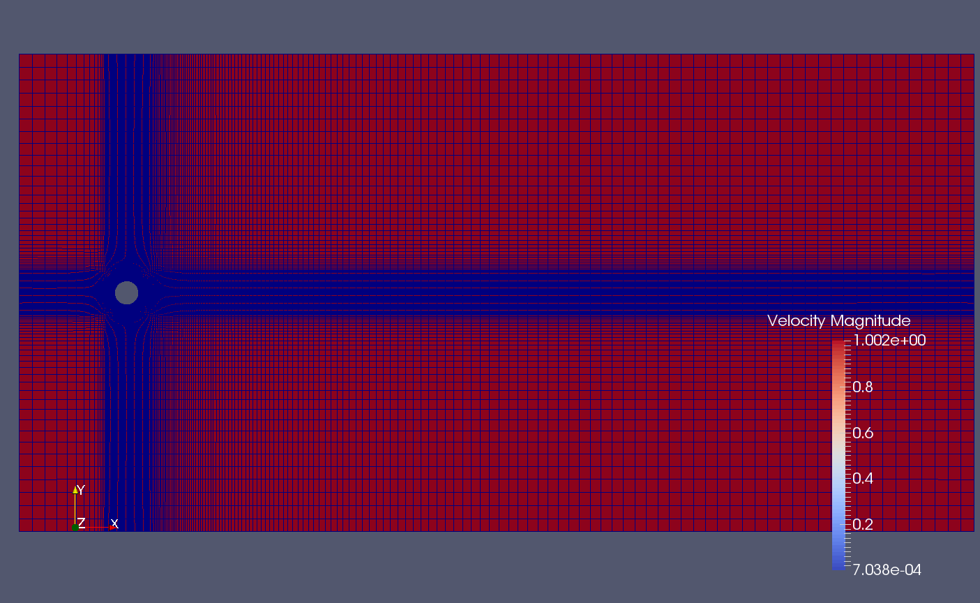
The cylinder diameter is not defined in the .ini file, but my mesh was generated so that D=1 and domain length -5<x<30 units. According to Paraview, your D=~285 and domain -2500<x<20000 units. Therefore, some of the values in the .ini file including the source terms should be scaled to match the dimensionless quantities. For example, now your Reynolds number is Re=1*285/0.008 = 35625 and one flow through would take 22500 time units. In the original file Re = 1*1/0.008=125 and flow through time 35 units.
-Niki
On 16/03/17 16:43, Zach Davis wrote:
Niki,
You aren’t seeing this in Paraview (see attached screenshot)? Also, where is the cylinder diameter defined within the *.ini file for this case. Are you referring to your setup of the source terms?
Best Regards,
Pointwise®, Inc.
Sr. Engineer, Sales & Marketing
213 South Jennings Avenue
Fort Worth, TX 76104-1107
E: zach....@pointwise.com
P: (817) 377-2807 x1202
F: (817) 377-2799
enc
<Mail Attachment.png>
Zach Davis
Niki Loppi
Hi Zach,
The backward Euler, bdf2, and bdf3 are backward difference
schemes, which are iterated explicitly in pseudo time. This is
because fully implicit approaches in high-order are unattractive
for GPUs due to their memory limitations. Therefore, the CFL is
limited by the stability of the explicit RK4. You have specified
the pseudo time step larger than the real time step, which is why
the simulation is almost guaranteed blow-up.
The source terms are not the issue. They are just used to prevent the reflection of the initial pseudo wave to make the initial transient phase faster and cleaner. You should be able to run the case without them, but then in the transient phase you are left with bouncing pressure waves. The coordinates +/-5 and +/-25 are from the origin, which is in the middle of the cylinder.
Yes, the paper says that the factor typically ranges from 1 to 4, but there is much more literature on this. Its appropriate value is affected by many different aspects, such as length scales in the simulation and the grid you are using. Moreover, it should have different values the viscous and advection dominated areas. Since the optimal value for beta should be temporally and spatially varying, the best option for now is just to find a good global value and stable time steps for each configuration heuristically. The value ac-zeta = 6 seemed to work fine in my configuration.
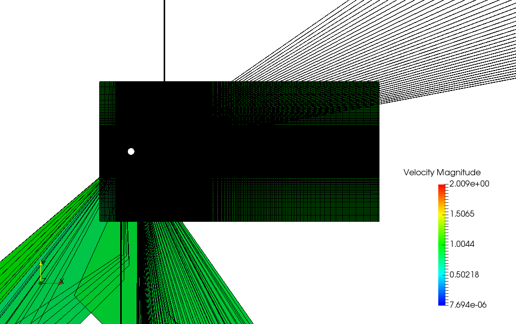
I managed to start the simulation with bdf2/rk4, ac-zeta = 4.0, dt = 0.0002, pseudo-dt = 0.0001 and 7th order flux anti-aliasing, but simulation blows up starting from the boundaries (picture attached). Just to be sure that the boundary definitions work correctly in the Pointwise pyfrm writer, could you write your mesh as Gmsh .msh and send it to me.
Thanks,
Niki
On Mar 16, 2017, at 12:47 PM, Niki Loppi <n.lo...@imperial.ac.uk> wrote:
Zach,
Yes, I saw that in your original .vtu file. However, when I started the simulation from scratch with your mesh, it did not reproduce the error. However, I did repartition it into two. Did you try it without partitioning?
The cylinder diameter is not defined in the .ini file, but my mesh was generated so that D=1 and domain length -5<x<30 units. According to Paraview, your D=~285 and domain -2500<x<20000 units. Therefore, some of the values in the .ini file including the source terms should be scaled to match the dimensionless quantities. For example, now your Reynolds number is Re=1*285/0.008 = 35625 and one flow through would take 22500 time units. In the original file Re = 1*1/0.008=125 and flow through time 35 units.
-Niki
On 16/03/17 16:43, Zach Davis wrote:
Niki,
You aren’t seeing this in Paraview (see attached screenshot)? Also, where is the cylinder diameter defined within the *.ini file for this case. Are you referring to your setup of the source terms?
Best Regards,
Pointwise®, Inc.
Sr. Engineer, Sales & Marketing
213 South Jennings Avenue
Fort Worth, TX 76104-1107
E: zach....@pointwise.com
P: (817) 377-2807 x1202
F: (817) 377-2799
enc
<Mail Attachment.png>
Zach Davis

|
Zach Davis Pointwise®, Inc. Sr. Engineer, Sales & Marketing 213 South Jennings Avenue Fort Worth, TX 76104-1107 E: zach....@pointwise.com P: (817) 377-2807 x1202 F: (817) 377-2799 |
Niki Loppi
Hi Zach,
The gmsh to .pyfrm converted mesh produced the same result as the
direct .pyrfm conversion, so the Pointwise writer is working fine.
Additionally, no anti-aliasing is needed, that was my mistake.
Sometimes anti-aliasing (over sampling) is needed for the
non-linear flux calculation in areas that are under-resolved. This
is not the case in this simulation and actually the resolution is
too high near the cylinder for P=4 which causes the major
limitation in the explicit pseudo-time step size. The high-order
CFL criterion is dependent on the polynomial order, which is why
you cant use the standard CFL expression. The solution is to make
the cylinder surface elements curved and increase their size to
efficiently use higher orders with less restrictive time-steps.
With P=3 you can get a stable combination with ac-zeta=4.0, dt = 0.001, pseudo-dt = 0.0005 which results in ~6 hour simulation with a single FirePro S10,000GPU. Please note that this artificial compressibility approach is formulated to leverage arithmetic capabilities of GPUs in order to make it competitive against codes that are based on global Poisson solve.
-Niki
--
You received this message because you are subscribed to the Google Groups "PyFR Mailing List" group.
To unsubscribe from this group and stop receiving emails from it, send an email to pyfrmailingli...@googlegroups.com.
To post to this group, send email to pyfrmai...@googlegroups.com.
Visit this group at https://groups.google.com/group/pyfrmailinglist.
For more options, visit https://groups.google.com/d/optout.
On Mar 20, 2017, at 11:50 AM, Niki Loppi <n.lo...@imperial.ac.uk> wrote:
Hi Zach,
The backward Euler, bdf2, and bdf3 are backward difference schemes, which are iterated explicitly in pseudo time. This is because fully implicit approaches in high-order are unattractive for GPUs due to their memory limitations. Therefore, the CFL is limited by the stability of the explicit RK4. You have specified the pseudo time step larger than the real time step, which is why the simulation is almost guaranteed blow-up.
The source terms are not the issue. They are just used to prevent the reflection of the initial pseudo wave to make the initial transient phase faster and cleaner. You should be able to run the case without them, but then in the transient phase you are left with bouncing pressure waves. The coordinates +/-5 and +/-25 are from the origin, which is in the middle of the cylinder.
Yes, the paper says that the factor typically ranges from 1 to 4, but there is much more literature on this. Its appropriate value is affected by many different aspects, such as length scales in the simulation and the grid you are using. Moreover, it should have different values the viscous and advection dominated areas. Since the optimal value for beta should be temporally and spatially varying, the best option for now is just to find a good global value and stable time steps for each configuration heuristically. The value ac-zeta = 6 seemed to work fine in my configuration.
I managed to start the simulation with bdf2/rk4, ac-zeta = 4.0, dt = 0.0002, pseudo-dt = 0.0001 and 7th order flux anti-aliasing, but simulation blows up starting from the boundaries (picture attached). Just to be sure that the boundary definitions work correctly in the Pointwise pyfrm writer, could you write your mesh as Gmsh .msh and send it to me.
Thanks,
Niki
On 17/03/17 18:16, Zach Davis wrote:
Hi Niki,
I’ve modified my 2_d cylinder mesh to use a diameter of 1. I’ve also brought in the control volume boundaries to align more with what was covered in the paper reference you provided. I’ve attached the mesh and configuration files I’m using in the hopes that you might have some time to help me troubleshoot, so I can better understand the process involved. The solver is diverging, and i’ve tried increasing the max number of sub-iterations, decreasing the time step, and so forth. I suspect it may have to do again with the source terms which I still don’t quite understand (are your +/-5 and +/-25 from the cylinder boundary or from the control volume boundaries?).
Also the paper suggests that the artificial compressibility factor they use is 1.25 and typically ranges from 1 to 4. Could you explain why you opted for a factor of 6? Lastly, is there a difference in how one should choose a time step and pseudo time step depending on whether the backward euler, bdf2, and bdf3 schemes are used? I assume the former is an explicit scheme; whereas, the latter two are implicit? Thanks!
Best Regards,
Zach
enc
On Mar 16, 2017, at 12:47 PM, Niki Loppi <n.lo...@imperial.ac.uk> wrote:
Zach,
Yes, I saw that in your original .vtu file. However, when I started the simulation from scratch with your mesh, it did not reproduce the error. However, I did repartition it into two. Did you try it without partitioning?
The cylinder diameter is not defined in the .ini file, but my mesh was generated so that D=1 and domain length -5<x<30 units. According to Paraview, your D=~285 and domain -2500<x<20000 units. Therefore, some of the values in the .ini file including the source terms should be scaled to match the dimensionless quantities. For example, now your Reynolds number is Re=1*285/0.008 = 35625 and one flow through would take 22500 time units. In the original file Re = 1*1/0.008=125 and flow through time 35 units.
-Niki
On 16/03/17 16:43, Zach Davis wrote:
Niki,
You aren’t seeing this in Paraview (see attached screenshot)? Also, where is the cylinder diameter defined within the *.ini file for this case. Are you referring to your setup of the source terms?
Best Regards,
Pointwise®, Inc.
Sr. Engineer, Sales & Marketing
213 South Jennings Avenue
Fort Worth, TX 76104-1107
E: zach....@pointwise.com
P: (817) 377-2807 x1202
F: (817) 377-2799
enc
<Mail Attachment.png>
On Mar 16, 2017, at 8:22 AM, Niki Loppi <n.lo...@imperial.ac.uk> wrote:
Hi Zach,
I tried running your case for couple of outputs and did not experience the odd behaviour in your .vtu file (attachment). However, in your mesh the dimensions are scaled differently. For instance, the cylinder diameter is D=~285, while the values in the .ini file are specified for D=1 used in my mesh.
Cheers,
Niki
On 15/03/17 20:27, Zach Davis wrote:
Hi Niki,
Thanks for the explanation. I’ll look into this method a bit further based on the paper reference you provided. Something seems to be amiss with solution files. I’ve attached the *.pyfrm *.vtu and *.ini files I have generated for this case; though, the mesh is one of my own creation. If someone could explain what’s happening with the *.vtu file based on the *.pyfrm mesh input, then that would be appreciated.
Best Regards,
![Pointwise, Inc.]()
Pointwise®, Inc.
Sr. Engineer, Sales & Marketing
213 South Jennings Avenue
Fort Worth, TX 76104-1107
E: zach....@pointwise.com
P: (817) 377-2807 x1202
F: (817) 377-2799
enc
On Mar 15, 2017, at 8:42 AM, Niki Loppi <n.lo...@imperial.ac.uk> wrote:
Hi Zach,
AC stands for the method of artificial compressibility. Instead of relying on a Poisson based projection, the system is driven towards a divergence free state by introducing artificial pressure waves through the continuity equation. The formulation preserves the hyperbolic nature of the system, but destroys the time accuracy, which is then recovered with dual time stepping. For the ac formulation you can refer to
http://www.sciencedirect.com/science/article/pii/S0021999116001686
The artificial compressibility factor ac-zeta is the coefficient of the fluxes in the continuity equation. This results in characteristics
V + c, V, V - c,
where c = sqrt(V^2 + ac-zeta) is the pseudo speed of sound. Thus, in the current implementation ac-zeta is the free parameter that is used to downscale the speed of the pseudo-waves to globally reduce the pseudo system stiffness. The parameter is something that one can experiment with, typical values varying from 1.25 - 10 times the freestream velocity. Currently, I am looking into making ac-zeta and pseudo-dt spatially and temporally varying.
The source terms specify a sponge region near the domain edges (|y|>5, x<-5, x>25) to damp the initial pressure wave that is generated when the simulation is started from scratch. Please note that the sponge turns off at t=5 because of the (1 - tanh(1.5*(t - 5.0)))*0.5 coefficient. You can see how the sponge works if you write the solution files before t=5.
The plugin [soln-plugin-pseudostats] is used to output the residual of the pseudo time problem to monitor the divergence. The [soln-plugin-residual] on the other hand computes the "residual" of two consecutive real time steps. The [soln-plugin-fluidforce] plugin can be used with the ac systems.
Coarsening the mesh and increasing the order is something that would be beneficial, especially when using a polynomial multigrid for accelerating the pseudo time problem. P-multigrid should be added in the next release.
Thanks,
Niki
On 14/03/17 23:37, Zach Davis wrote:
Tuesday, 14 March 2017
Peter & Freddie,
I believe the mesh export issue from Pointwise using the PyFR exporter has been resolved in PyFR 1.6. I still seem to have issues running using the OpenCL backend which persistently complains about an invalid workgroup size. It use to work at one point, but something has changed in the intervening releases which is causing problems for me at least. I’ve tried adjusting the values per Freddie’s guidance to no avail. He also suggested a tool that might be helpful in determining the appropriate workgroup size needed for my card. Unfortunately that tool seems to be NVIDIA card specific requiring installation of NVIDIA software that won’t run on my machine. I’m using an AMD card instead, and the tool won’t compile due to missing dependencies. It’s not a pressing matter, but just something that I thought you both might want to be aware of.
Nikki,
I’ve looked over your incompressible 2d-cylinder case, and I was wondering if you could elaborate a bit, or point me to some reference, about how you came up with the source terms you’re using in the input file. It also appears that the [soln-plugin-pseudostats] is used in place of the [soln-plugin-residual] namelist for incompressible cases—is that right? Does the [soln-plugin-fluidforce] namelist still work for the ac-navier-stokes solver? Another question if you don’t mind—what is this artificial compressibility factor, ac-zeta and why is value of 6.0 used? Oh, and what does the ac prefix stand for? Thanks!
I think it would be interesting to see how coarse of a higher-order mesh could be made for this case while increasing the polynomial solution basis such that you essentially recover the linear mesh spacing in each element, and see if you could capture one or more vortices within a single element with any noticeable diffusion over time.
Best Regards,
![Pointwise, Inc.]()
Pointwise®, Inc.
Sr. Engineer, Sales & Marketing
213 South Jennings Avenue
Fort Worth, TX 76104-1107
E: zach....@pointwise.com
P: (817) 377-2807 x1202
F: (817) 377-2799
<0.4.png>
Zach Davis
|
|
Zach Davis
Pointwise®, Inc. Sr. Engineer, Sales & Marketing 213 South Jennings Avenue Fort Worth, TX 76104-1107 E: zach....@pointwise.com P: (817) 377-2807 x1202 F: (817) 377-2799 |
Niki Loppi
Hi Zach,
You mean the source terms? On a GPU they seem to increase the simulation time by less than 8%. Since they turn off at t=5 anyway, you can restart the simulation without them from 5.00.pyfrs to reduce the cost.
Turning the surf-flux anti-aliasing on and increasing the
quad-deg order under the surface element-types is equivalent to
sub-sampling the flux polynomial at quadrature points along the
linear interfaces for more accurate integration. The curvature of
elements is achieved with polynomial representations defined by
shape points and that information comes from the high-order mesh.
The algorithm is formulated to be as compute intensive as possible to leverage the arithmetic capabilities of GPUs/co-processors. Other incompressible approaches normally rely on (partly) implicit time stepping and a global matrix inversion which makes them memory intensive/bandwidth bound and thereby less attractive for GPUs. You can find more about the GPU motivation in the original PyFR paper.
http://www.sciencedirect.com/science/article/pii/S0010465514002549
Niki
Zach Davis
|
|
Zach Davis
Pointwise®, Inc. Sr. Engineer, Sales & Marketing 213 South Jennings Avenue Fort Worth, TX 76104-1107 E: zach....@pointwise.com P: (817) 377-2807 x1202 F: (817) 377-2799 |
Loppi, Niki
Zach Davis
Niki Loppi
Hi Zach,
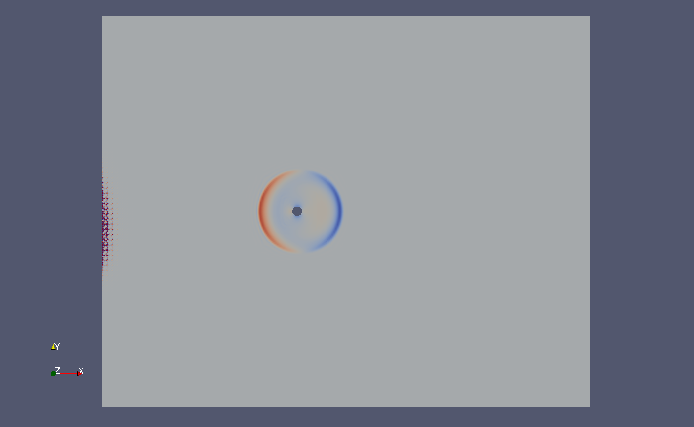
The setup should be fine. Have tried to run the simulation further? It looks like it is just about to start shedding. For comparison https://www.youtube.com/watch?v=EOuOZxqcOng
Niki
--
You received this message because you are subscribed to the Google Groups "PyFR Mailing List" group.
To unsubscribe from this group and stop receiving emails from it, send an email to pyfrmailingli...@googlegroups.com.
To post to this group, send email to pyfrmai...@googlegroups.com.
Visit this group at https://groups.google.com/group/pyfrmailinglist.
For more options, visit https://groups.google.com/d/optout.
On Mar 22, 2017, at 5:46 PM, Loppi, Niki <n.lo...@imperial.ac.uk> wrote:
Hi Zach,
If you only use the surf-flux anti-aliasing, defining the quadrature degree for the line interfaces is sufficient. If you use the other anti-aliasing options (flux, div-flux) you need to specify it for the quad element type as well.
Yes, as far I as I’m aware, that is how the high-order meshes work in PyFR.
-Niki
On 21 Mar 2017, at 20:44, Zach Davis <zda...@pointwise.com> wrote:
Hi Niki,
Yes, I was referring to the source terms. If I turn on surf-flux anti-aliasing, do I need to define the quadrature degree order and quadrature rule type for both the line interfaces and quad element type, or is defining it for only the quad element type necessary?
Are you saying when we send you higher order meshes, the additional “shape points” created in elevating the mesh order are then used to define a polynomial that PyFR in turn uses to represent the curvature of the element?
Best Regards,
Pointwise®, Inc.
Sr. Engineer, Sales & Marketing
213 South Jennings Avenue
Fort Worth, TX 76104-1107
E: zach....@pointwise.com
P: (817) 377-2807 x1202
F: (817) 377-2799


On Mar 21, 2017, at 12:38 PM, Niki Loppi <n.lo...@imperial.ac.uk> wrote:
Hi Zach,
You mean the source terms? On a GPU they seem to increase the simulation time by less than 8%. Since they turn off at t=5 anyway, you can restart the simulation without them from 5.00.pyfrs to reduce the cost.
Turning the surf-flux anti-aliasing on and increasing the quad-deg order under the surface element-types is equivalent to sub-sampling the flux polynomial at quadrature points along the linear interfaces for more accurate integration. The curvature of elements is achieved with polynomial representations defined by shape points and that information comes from the high-order mesh.
The algorithm is formulated to be as compute intensive as possible to leverage the arithmetic capabilities of GPUs/co-processors. Other incompressible approaches normally rely on (partly) implicit time stepping and a global matrix inversion which makes them memory intensive/bandwidth bound and thereby less attractive for GPUs. You can find more about the GPU motivation in the original PyFR paper.
http://www.sciencedirect.com/science/article/pii/S0010465514002549
Niki
On 20/03/17 21:57, Zach Davis wrote:
Hi Niki,
So, with the artificial compressibility terms turned on, the simulation would require about 40 hours on 4 cores using the OpenMP backend with the new values for dt and pseudo-dt. Turning them off requires only 15 hours to run the solver for a 3rd order solution. Are they necessary? Is there more I can read about why this formulation of yours favors GPUs?
I’m getting to curving in upcoming runs, but wanted a linear mesh to begin with. for comparison This leads into another question I have. I know PyFR inserts solution points via quadrature rules for each element type which are primarily used in integration over the element. Does PyFR also insert points along the interfaces of the elements as well for computing fluxes? What if these points already exists as in when we elevate the order of the mesh?
Best Regards,
Pointwise®, Inc.
Sr. Engineer, Sales & Marketing
213 South Jennings Avenue
Fort Worth, TX 76104-1107
E: zach....@pointwise.com
P: (817) 377-2807 x1202
F: (817) 377-2799
On Mar 20, 2017, at 3:40 PM, Niki Loppi <n.lo...@imperial.ac.uk> wrote:
Hi Zach,
The gmsh to .pyfrm converted mesh produced the same result as the direct .pyrfm conversion, so the Pointwise writer is working fine. Additionally, no anti-aliasing is needed, that was my mistake.
Sometimes anti-aliasing (over sampling) is needed for the non-linear flux calculation in areas that are under-resolved. This is not the case in this simulation and actually the resolution is too high near the cylinder for P=4 which causes the major limitation in the explicit pseudo-time step size. The high-order CFL criterion is dependent on the polynomial order, which is why you cant use the standard CFL expression. The solution is to make the cylinder surface elements curved and increase their size to efficiently use higher orders with less restrictive time-steps.
With P=3 you can get a stable combination with ac-zeta=4.0, dt = 0.001, pseudo-dt = 0.0005 which results in ~6 hour simulation with a single FirePro S10,000GPU. Please note that this artificial compressibility approach is formulated to leverage arithmetic capabilities of GPUs in order to make it competitive against codes that are based on global Poisson solve.
-Niki
On 20/03/17 17:39, Zach Davis wrote:
Hi Niki,
Thanks for catching my time stepping error. I transposed the time step values that were reported in the paper incorrectly. In choosing an appropriate time step, the CFL criteria seems to suggest that I need to select something less than1.0*(min dS spacing/vel). Since I’m normalizing the u velocity to 1.0, then I think my time step should correspond directly to my minimum dS spacing. I can see what that minimum spacing is directly in Pointwise (~0.0583), but it appears that you need to back off from that substantially.
If I try to run this on 4 cores using the OpenMP backend, PyFR estimates that it would take about 375 hours to simulate 60 seconds. This lead to my earlier comment about this taking awhile. I would try using the OpenCL backend, but it currently isn’t working for me. I also think this mesh is small enough that I wouldn’t notice much of speedup difference.
I don’t have any understanding of what antialiasing accomplishes in PyFR, or how to set it up appropriately. My initial impression was that it would be used in conjunction with shock capturing simulations in order to smooth the gradients across elements in the vicinity of a shock or other strong discontinuity in the control volume. If you’re employing it for this case, then perhaps my assumption is wrong. Are there references you can point me to that discuss this topic a bit further?
The Gmsh file for this mesh is attached. Thanks so much for working through this with me!
Best Regards,
Pointwise®, Inc.
Sr. Engineer, Sales & Marketing
213 South Jennings Avenue
Fort Worth, TX 76104-1107
E: zach....@pointwise.com
P: (817) 377-2807 x1202
F: (817) 377-2799
enc
Best Regards,
Pointwise®, Inc.
Sr. Engineer, Sales & Marketing
213 South Jennings Avenue
Fort Worth, TX 76104-1107
E: zach....@pointwise.com
P: (817) 377-2807 x1202
F: (817) 377-2799
enc
<Mail Attachment.png>
On Mar 16, 2017, at 8:22 AM, Niki Loppi <n.lo...@imperial.ac.uk> wrote:
Hi Zach,
I tried running your case for couple of outputs and did not experience the odd behaviour in your .vtu file (attachment). However, in your mesh the dimensions are scaled differently. For instance, the cylinder diameter is D=~285, while the values in the .ini file are specified for D=1 used in my mesh.
Cheers,
Niki
On 15/03/17 20:27, Zach Davis wrote:
Hi Niki,
Thanks for the explanation. I’ll look into this method a bit further based on the paper reference you provided. Something seems to be amiss with solution files. I’ve attached the *.pyfrm *.vtu and *.ini files I have generated for this case; though, the mesh is one of my own creation. If someone could explain what’s happening with the *.vtu file based on the *.pyfrm mesh input, then that would be appreciated.
Best Regards,
![Pointwise, Inc.]()
Pointwise®, Inc.
Sr. Engineer, Sales & Marketing
213 South Jennings Avenue
Fort Worth, TX 76104-1107
E: zach....@pointwise.com
P: (817) 377-2807 x1202
F: (817) 377-2799
enc
On Mar 15, 2017, at 8:42 AM, Niki Loppi <n.lo...@imperial.ac.uk> wrote:
Hi Zach,
AC stands for the method of artificial compressibility. Instead of relying on a Poisson based projection, the system is driven towards a divergence free state by introducing artificial pressure waves through the continuity equation. The formulation preserves the hyperbolic nature of the system, but destroys the time accuracy, which is then recovered with dual time stepping. For the ac formulation you can refer to
http://www.sciencedirect.com/science/article/pii/S0021999116001686
The artificial compressibility factor ac-zeta is the coefficient of the fluxes in the continuity equation. This results in characteristics
V + c, V, V - c,
where c = sqrt(V^2 + ac-zeta) is the pseudo speed of sound. Thus, in the current implementation ac-zeta is the free parameter that is used to downscale the speed of the pseudo-waves to globally reduce the pseudo system stiffness. The parameter is something that one can experiment with, typical values varying from 1.25 - 10 times the freestream velocity. Currently, I am looking into making ac-zeta and pseudo-dt spatially and temporally varying.
The source terms specify a sponge region near the domain edges (|y|>5, x<-5, x>25) to damp the initial pressure wave that is generated when the simulation is started from scratch. Please note that the sponge turns off at t=5 because of the (1 - tanh(1.5*(t - 5.0)))*0.5 coefficient. You can see how the sponge works if you write the solution files before t=5.
The plugin [soln-plugin-pseudostats] is used to output the residual of the pseudo time problem to monitor the divergence. The [soln-plugin-residual] on the other hand computes the "residual" of two consecutive real time steps. The [soln-plugin-fluidforce] plugin can be used with the ac systems.
Coarsening the mesh and increasing the order is something that would be beneficial, especially when using a polynomial multigrid for accelerating the pseudo time problem. P-multigrid should be added in the next release.
Thanks,
Niki
On 14/03/17 23:37, Zach Davis wrote:
Tuesday, 14 March 2017
Peter & Freddie,
I believe the mesh export issue from Pointwise using the PyFR exporter has been resolved in PyFR 1.6. I still seem to have issues running using the OpenCL backend which persistently complains about an invalid workgroup size. It use to work at one point, but something has changed in the intervening releases which is causing problems for me at least. I’ve tried adjusting the values per Freddie’s guidance to no avail. He also suggested a tool that might be helpful in determining the appropriate workgroup size needed for my card. Unfortunately that tool seems to be NVIDIA card specific requiring installation of NVIDIA software that won’t run on my machine. I’m using an AMD card instead, and the tool won’t compile due to missing dependencies. It’s not a pressing matter, but just something that I thought you both might want to be aware of.
Nikki,
I’ve looked over your incompressible 2d-cylinder case, and I was wondering if you could elaborate a bit, or point me to some reference, about how you came up with the source terms you’re using in the input file. It also appears that the [soln-plugin-pseudostats] is used in place of the [soln-plugin-residual] namelist for incompressible cases—is that right? Does the [soln-plugin-fluidforce] namelist still work for the ac-navier-stokes solver? Another question if you don’t mind—what is this artificial compressibility factor, ac-zeta and why is value of 6.0 used? Oh, and what does the ac prefix stand for? Thanks!
I think it would be interesting to see how coarse of a higher-order mesh could be made for this case while increasing the polynomial solution basis such that you essentially recover the linear mesh spacing in each element, and see if you could capture one or more vortices within a single element with any noticeable diffusion over time.
Best Regards,
![Pointwise, Inc.]()
Pointwise®, Inc.
Sr. Engineer, Sales & Marketing
213 South Jennings Avenue
Fort Worth, TX 76104-1107
E: zach....@pointwise.com
P: (817) 377-2807 x1202
F: (817) 377-2799
Zach Davis
|
|
Zach Davis
Pointwise®, Inc. Sr. Engineer, Sales & Marketing 213 South Jennings Avenue Fort Worth, TX 76104-1107 E: zach....@pointwise.com P: (817) 377-2807 x1202 F: (817) 377-2799 |