New semTools function for testing measurement equivalence / invariance

[Terrence Jorgensen]

For the past few years, there have been 3 separate functions for automatically testing the omnibus null hypotheses of measurement invariance, each under very constrained conditions (e.g., simple structure, first-order measurement). 

• measurementInvariance(): only for numeric indicators, only tests across multiple groups
• measurementInvarianceCat(): only for ordered indicators, only tests across multiple groups
• longInvariance(): only for numeric indicators of 1 (repeatedly measured) factor, only tests across repeated measures

In the next version of semTools, these functions will still available, but they have been deprecated.  

The new function measEq.syntax() addresses all of the above limitations by writing lavaan model syntax and (optionally) fitting the model to data.  By specifying a configural model with minimal syntax (i.e., the pattern of factor loadings), users can set arguments to specify models with invariance constraints imposed on any measurement and/or structural parameters across any combination of multiple groups and/or repeated measures.  The configural model may have complex structure (i.e., cross-loadings and residual covariances are allowed), higher-order factors, and any combination of numeric and ordered indicators.  Different repeatedly measured factors do not need to all be measured on the same number of occasions, nor do the same indicators even need to be measured on all occasions (e.g., if some test items are replaced when measuring abilities at later ages).  Beyond the choice between std.lv = TRUE or FALSE in the previous functions, users can also choose effects-coding to identify common-factor distributions (except in models with cross-loadings, such as bifactor models).  Users can also choose between 4 different methods for identifying the latent item-response distributions underlying any ordered indicators, no longer being confined to use the Millsap & Tein (2004) recommendations implemented in measurementInvarianceCat().  The measEq.syntax() function (and now the compareFit() function) can also be applied to lavaan.mi objects, if users fit lavaan models to multiple imputations.  If a user still has a more complex situation than can be automated using the measEq.syntax() function, it is still possible to specify a model with similar needs, then print the lavaan model syntax and edit it manually to fit the desired model.

I encourage anyone who has had difficulty using the previous invariance-testing functions to try using this, and please let me know if there are any difficulties.  Users can install the development version of semTools and find examples on the help page to get started:

devtools::install_github("simsem/semTools/semTools")
library(semTools)
?measEq.syntax

The help page examples show how the user can mimic the Console output of the previous functions by looping over a sequence of constraints, saving the fitted models in a list, and comparing their fit using the compareFit() function.  Eventually, I will write an interactive wrapper function to do this, integrating follow-up tests rather than only providing omnibus tests that assume all previous levels of invariance are tenable.  But that will only be possible after updating the existing partialInvariance() function to work in this new framework, and I probably will not have time to work on that soon. 

Thanks for any feedback (please post here so others can benefit),

Terrence D. Jorgensen

Postdoctoral Researcher, Methods and Statistics

Research Institute for Child Development and Education, the University of Amsterdam

UvA web page: http://www.uva.nl/profile/t.d.jorgensen

[Giacomo Mason]

Thank you for the hard work Terrence, I'll try this out soon.

Giacomo

[Giacomo Mason]

I can't seem to be able to install semTools from GitHub using devtools. Is that possible?

Best,

G

On Sunday, August 26, 2018 at 11:02:43 PM UTC+1, Terrence Jorgensen wrote:

[Terrence Jorgensen]

I can't seem to be able to install semTools from GitHub using devtools

My colleague was able to install it.  Do you have the latest R (3.5.1) and development version of lavaan (0.6-3.1295 installed?

http://lavaan.ugent.be/development.html

And is devtools installed?

library(devtools)

[Carlos Lemos]

I can't thank you enough for this, Terrence!

I had a hard time implementing the Wu & Estabrook procedure following your advice, and I can imagine the amount of expertise and work required to write this function.

I will certainly try it and give feedback.

Best regards,

Carlos

--
You received this message because you are subscribed to the Google Groups "lavaan" group.
To unsubscribe from this group and stop receiving emails from it, send an email to lavaan+un...@googlegroups.com.
To post to this group, send email to lav...@googlegroups.com.
Visit this group at https://groups.google.com/group/lavaan.
For more options, visit https://groups.google.com/d/optout.

[Carlos Lemos]

Hi again Terrence,

I’m trying to use the new measEq.Syntax() function to study measurement invariance on the ISSP religion data. Here is the structure of the data frame:

> str(df)

'data.frame':   35198 obs. of  20 variables:

 $ V28         : Ord.factor w/ 3 levels "I don't believe in God"<..: 3 3 2 2 2 2 2 2 2 2 ...

 $ V30         : Ord.factor w/ 4 levels "No, definitely not"<..: 2 4 2 2 4 NA 1 NA 2 1 ...

 $ V31         : Ord.factor w/ 4 levels "No, definitely not"<..: 2 4 2 1 NA 1 1 NA 1 3 ...

 $ V32         : Ord.factor w/ 4 levels "No, definitely not"<..: 2 2 2 1 NA 1 1 1 2 3 ...

 $ V33         : Ord.factor w/ 4 levels "No, definitely not"<..: 3 4 2 1 1 3 1 2 2 3 ...

 $ V35         : Ord.factor w/ 5 levels "Strongly disagree"<..: 2 5 3 1 2 NA 1 3 3 NA ...

 $ V37         : Ord.factor w/ 5 levels "Strongly disagree"<..: 3 2 3 1 1 1 1 3 3 NA ...

 $ V46         : Ord.factor w/ 4 levels "Never"<"Yearly"<..: 4 3 3 1 2 2 3 2 1 3 ...

 $ V47         : Ord.factor w/ 4 levels "Never"<"Yearly"<..: 3 NA 2 1 2 NA 1 1 1 3 ...

 $ V48         : Ord.factor w/ 4 levels "Never"<"Yearly"<..: 4 4 2 1 2 4 3 1 2 3 ...

 $ V49         : Ord.factor w/ 5 levels "Never"<"Yearly"<..: 4 1 2 1 1 1 1 1 1 3 ...

 $ V50         : Ord.factor w/ 5 levels "Never"<"Yearly"<..: 2 1 1 2 1 1 1 1 1 2 ...

 $ V51         : Ord.factor w/ 5 levels "Highly non-religious"<..: 4 1 2 1 1 4 2 2 2 2 ...

 $ ATTEND      : Ord.factor w/ 4 levels "Never"<"Yearly"<..: 4 1 2 1 1 2 1 1 1 3 ...

 $ AGE         : Ord.factor w/ 5 levels "0-24"<"25-44"<..: 4 2 2 2 2 3 3 3 3 3 ...

 $ SEX         : Factor w/ 2 levels "Male","Female": 2 2 1 1 1 1 2 1 1 2 ...

 $ DEGREE      : Ord.factor w/ 6 levels "No formal qualification"<..: 2 4 4 6 4 6 3 3 4 3 ...

 $ RELIGGRP    : Factor w/ 5 levels "No religion",..: 2 2 4 1 1 1 2 1 1 2 ...

 $ COUNTRY.NAME: Factor w/ 26 levels "AU-Australia",..: 2 3 4 5 7 8 9 12 13 17 ...

 $ YEAR        : Ord.factor w/ 1 level "2008": 1 1 1 1 1 1 1 1 1 1 ...

>

> 

 

I defined the following items as ordinal and converted to numeric, and for simplicity I used “SEX” as the group factor (just two levels):

> indicators <- c("V28", "V30", "V31", "V32", "V33",        

+                 "V35", "V37",         

+                 "V46", "V47", "V48", "V49", "V50",        

+                 "V51", "ATTEND")

> for (ind in indicators) {

+   df[,ind] <- as.numeric(df[,ind])

+ }

> group <- "SEX"

> 

I now tried to compute a configural model, first with “cfa” and then with “measEq.syntax”, for a single factor:

> model <- "afterlife =~ V30 + V31 + V32 + V33"

> # CONFIGURAL

> config <- cfa(model, data = df, ordered = indicators, parameterization = "theta",

+               estimator = "WLSMV", group = group, group.equal = "")

> config <- measEq.syntax(model, data = df, ordered = indicators, parameterization = "theta",

+                         ID.fac = "std.lv", ID.cat = "Wu.Estabrook.2016", estimator = "WLSMV",

+                         group = group, group.equal = "", return.fit = TRUE)

Error in specify[[1]][RR, CC] : subscript out of bounds

> 

The first runs, the second gives an error. However, if I define this 2-factor model:

model <- "afterlife =~ V30 + V31 + V32 + V33

          belief.God =~ V28 + V35 + V37"

 

it runs OK:

> config <- cfa(model, data = df, ordered = indicators, parameterization = "theta",

+               estimator = "WLSMV", group = group, group.equal = "")

> config <- measEq.syntax(model, data = df, ordered = indicators, parameterization = "theta",

+                         ID.fac = "std.lv", ID.cat = "Wu.Estabrook.2016", estimator = "WLSMV",

+                         group = group, group.equal = "", return.fit = TRUE)

> 

What am I doing wrong?

I proceeded to compute a model with constrained thresholds and loadings, which tests for metric invariance (scales of both latent response variables and factors fixed across groups):

> metric <- measEq.syntax(model, data = df, ordered = indicators, parameterization = "theta",

+                         ID.fac = "std.lv", ID.cat = "Wu.Estabrook.2016", estimator = "WLSMV",

+                         group = group, group.equal = c("thresholds","loadings"),

                          return.fit = TRUE)

> 

and it runs OK and has good fit (cfi = 0.99936, rmsea = 0.03707745, srmr = 0.0183). I inspected the parameter table and checked that the identification conditions in eq. (19) of Wu and Estabrook are nicely in place (thank you very much for this!!!). However, when I check the estimator:

> unlist(lavInspect(metric, what = "Options"))["estimator"]

estimator

   "DWLS"

> 

I don’t get “WLSMV”, which is recommended for MGCFA with ordinal variables.

Finally, I have another doubt. I’m trying to run multiple imputed files with measEq.syntax(), but since this takes a long time with “mice”, I thought of saving the imputed data frames in a “mids” object and then running the analysis. However, I could not figure out how to do this with the help page of measEq.syntax().

Thank you very much once again for writing this wonderful function and for your help and attention.

Sincerely,

 

Carlos M. Lemos

Em seg, 27 de ago de 2018 às 00:02, Terrence Jorgensen <tjorge...@gmail.com> escreveu:

[dvillarre...@gmail.com]

Hi Terrence,

Thank you very much for this function.

I have a problem running my model, it is a longitudinal invariance analysis with categorical variables.

They are a total of seven measurements (DEP0 to DEP6), with nine items in each measurement. The items score from 0 to 3, however, in some follow-ups the items only reach scores from 0 to 2.

 

 

model <- "

DEP0 =~ f0V1 + f0V2 + f0V3 + f0V4 + f0V5 + f0V6 + f0V7 + f0V8 + f0V9
DEP1 =~ f1V1 + f1V2 + f1V3 + f1V4 + f1V5 + f1V6 + f1V7 + f1V8 + f1V9
DEP2 =~ f2V1 + f2V2 + f2V3 + f2V4 + f2V5 + f2V6 + f2V7 + f2V8 + f2V9
DEP3 =~ f3V1 + f3V2 + f3V3 + f3V4 + f3V5 + f3V6 + f3V7 + f3V8 + f3V9
DEP4 =~ f4V1 + f4V2 + f4V3 + f4V4 + f4V5 + f4V6 + f4V7 + f4V8 + f4V9
DEP5 =~ f5V1 + f5V2 + f5V3 + f5V4 + f5V5 + f5V6 + f5V7 + f5V8 + f5V9
DEP6 =~ f6V1 + f6V2 + f6V3 + f6V4 + f6V5 + f6V6 + f6V7 + f6V8 + f6V9
"


var0 <- c("f0V1", "f0V2", "f0V3", "f0V4", "f0V5", "f0V6", "f0V7", "f0V8", "f0V9")
var1 <- c("f1V1", "f1V2", "f1V3", "f1V4", "f1V5", "f1V6", "f1V7", "f1V8", "f1V9")
var2 <- c("f2V1", "f2V2", "f2V3", "f2V4", "f2V5", "f2V6", "f2V7", "f2V8", "f2V9")    
var3 <- c("f3V1", "f3V2", "f3V3", "f3V4", "f3V5", "f3V6", "f3V7", "f3V8", "f3V9")
var4 <- c("f4V1", "f4V2", "f4V3", "f4V4", "f4V5", "f4V6", "f4V7", "f4V8", "f4V9")
var5 <- c("f5V1", "f5V2", "f5V3", "f5V4", "f5V5", "f5V6", "f5V7", "f5V8", "f5V9")
var6 <- c("f6V1", "f6V2", "f6V3", "f6V4", "f6V5", "f6V6", "f6V7", "f6V8", "f6V9")
 

longFacNames <- list(FU = c("DEP0","DEP1","DEP2","DEP3","DEP4","DEP5","DEP6"))



syntax.config <- measEq.syntax(configural.model = model, data = DEP_SAL, parameterization = "theta",
                        ID.fac = "std.lv", ID.cat = "millsap", estimator = "WLSMV",
                        return.fit = TRUE, longFacNames=longFacNames,
                        ordered = c("f0V1", "f0V2", "f0V3", "f0V4", "f0V5", "f0V6", "f0V7", "f0V8", "f0V9",
                                    "f1V1", "f1V2", "f1V3", "f1V4", "f1V5", "f1V6", "f1V7", "f1V8", "f1V9",
                                    "f2V1", "f2V2", "f2V3", "f2V4", "f2V5", "f2V6", "f2V7", "f2V8", "f2V9",
                                    "f3V1", "f3V2", "f3V3", "f3V4", "f3V5", "f3V6", "f3V7", "f3V8", "f3V9",
                                    "f4V1", "f4V2", "f4V3", "f4V4", "f4V5", "f4V6", "f4V7", "f4V8", "f4V9",
                                    "f5V1", "f5V2", "f5V3", "f5V4", "f5V5", "f5V6", "f5V7", "f5V8", "f5V9",
                                    "f6V1", "f6V2", "f6V3", "f6V4","f6V5", "f6V6", "f6V7", "f6V8", "f6V9"))

 

cat(as.character(syntax.config))


summary(syntax.config, fit.measures=TRUE, standardized=TRUE)  

When I mail the analysis I get this error

Error in lav_samplestats_step1(Y = Data, ov.names = ov.names, ov.types = ov.types,  :
  lavaan ERROR: some categories of variable `f0V8' are empty in group 1; frequencies are [1670 45 43 0]

[Terrence Jorgensen]

I defined the following items as ordinal and converted to numeric

That is not necessary. If the ordered variables are already declared as ordered in the data.frame, then you don't even need to use the ordered= argument.

http://lavaan.ugent.be/tutorial/cat.html

Error in specify[[1]][RR, CC] : subscript out of bounds

I'm glad you tried it with both a 1-factor and 2-factor model. That helped me locate the source of the error and add a check so that syntax is only written for factor covariances if there are any.  If you install the development version of semTools again, it should work

when I check the estimator:

> unlist(lavInspect(metric, what = "Options"))["estimator"]

estimator

   "DWLS"

> 

I don’t get “WLSMV”, which is recommended for MGCFA with ordinal variables.

WLSMV is not an estimator.  That is just the shortcut for setting estimator = "DWLS", test = "scaled.shifted", and se = "robust.sem".  Nothing to do with this function; check the result for config when fitted with cfa().

Finally, I have another doubt. I’m trying to run multiple imputed files with measEq.syntax(), but since this takes a long time with “mice”, I thought of saving the imputed data frames in a “mids” object and then running the analysis. However, I could not figure out how to do this with the help page of measEq.syntax().

Yes, you should impute your data first so you are not wasting time repeating the imputation process before each analysis.  If you fit the configural model to the imputed data with runMI(), you can submit that object to measEq.syntax().  Here is an example.

set.seed(12345)
HSMiss <- HolzingerSwineford1939[ , paste("x", 1:9, sep = "")]
HSMiss$x5 <- ifelse(HSMiss$x1 <= quantile(HSMiss$x1, .3), NA, HSMiss$x5)
HSMiss$x9 <- ifelse(is.na(HSMiss$x5), NA, HSMiss$x9)
HSMiss$school <- HolzingerSwineford1939$school
HS.amelia <- amelia(HSMiss, m = 20, noms = "school")
imps <- HS.amelia$imputations

HS.model <- '
visual  =~ x1 + a*x2 + b*x3
textual =~ x4 + x5 + x6
speed   =~ x7 + x8 + x9
ab := a*b
'
mgfit1 <- cfa.mi(HS.model, data = imps, std.lv = TRUE, group = "school")

syntax.mi <- measEq.syntax(configural.model = mgfit1, group = "school",
                           group.equal = c("loadings","intercepts"))
cat(as.character(syntax.mi))
summary(syntax.mi)

## return fit
fit.mi <- measEq.syntax(configural.model = mgfit1, group = "school",
                        group.equal = c("loadings","intercepts"),
                        return.fit = TRUE)
summary(fit.mi)

Terrence D. Jorgensen

Postdoctoral Researcher, Methods and Statistics

Research Institute for Child Development and Education, the University of Amsterdam

http://www.uva.nl/profile/t.d.jorgensen

[Terrence Jorgensen]

When I mail the analysis I get this error

Error in lav_samplestats_step1(Y = Data, ov.names = ov.names, ov.types = ov.types,  :
  lavaan ERROR: some categories of variable `f0V8' are empty in group 1; frequencies are [1670 45 43 0]

The source of the error is clearly noted in the error message, and it has nothing to do with the syntax-writing function.  If you fit the configural model yourself with cfa(), you will notice the same error occurs.  

Terrence D. Jorgensen

Postdoctoral Researcher, Methods and Statistics

Research Institute for Child Development and Education, the University of Amsterdam

http://www.uva.nl/profile/t.d.jorgensen

[Carlos Lemos]

Hi again Terrence,

I'm glad that my feedback was somehow useful to you. I will reinstall semTools and retry.

Thank you very much for also clarifying my confusion about WLSMV and for sending the example on combining cfa.mi() with measEq.syntax(). I will make sure to set std.lv = TRUE in the call to cfa.mi (I missed that in my example) and then ID.fac = "std.lv" and ID.cat = "Wu.Estabrook.2016" in the call to measEq.syntax().

Best regards,

Carlos

[Una]

Thank you for all the work, and making our work simpler. I am now trying the function to test longitudinal variance, and I'm having problems with the long.partial argument.

This is the syntax:

mi.i<-measEq.syntax(ep.m, data= data,estimator="MLM", meanstructure=TRUE, int.lv.free=TRUE, auto.fix.first=T , orthogonal=T,
                    ID.fac="auto.fix.first",  return.fit = TRUE,
                    longFacNames =  list(X = c("X1","X2")), auto=T,
                    long.equal=c("loadings","intercepts"), long.partial = c("x2.1 ~ 1","x2.2 ~ 1"))

And this is the warning message:

Warning message: In if (long.partial == "") { : the condition has length > 1 and only the first element will be used

If I use only long.partial="x2 ~ 1", it doesn't give a warning message, but it still equals the intercepts.

Hope this feedback helps...

Kind regards,

Una

[Terrence Jorgensen]

long.partial = c("x2.1 ~ 1","x2.2 ~ 1"))

And this is the warning message:

Warning message: In if (long.partial == "") { : the condition has length > 1 and only the first element will be used

If I use only long.partial="x2 ~ 1", it doesn't give a warning message, but it still equals the intercepts.

 

I fixed the warning by checking the length too, but it is not something that would have actually led to a problem for anyone.

The problem (I am guessing) is that you are using actual observed-variable names in the vector: Are x2.1 and x2.2 the same variable measured at times 1 and 2, respectively?  

When you use long.partial="x2 ~ 1", that seems to refer to a name that you give to the observed variables x2.1 and x2.2 that are repeatedly measured (i.e., x2 itself is not a variable in your data set, right?).  In order to do that, you need to tell the function that "x2" refers to c("x2.1","x2.2") using the longIndNames= argument, which works the same way longFacNames= does.  As described in the "Repeated Measures" part of the Details section in the help page, if you don't make your own longIndNames, the default will be to assign automated labels based on the order, using the factor name.  So, since your longitudinal factor is named "X", the automated indicator name would probably be "._X_ind.2" (assuming it is the second indicator specified after =~ both times).  But of course I would recommend assigning your own longIndNames so you can use sensible names in long.partial=.

[Una]

Thank you for the feedback, I did judge wrongly how the automated labels would look like. If I understood correctly, in long.partial I can not use actual observed-variables names (which were in my case  x2.1  and  x2.2, the same variable measured two times, as you supposed) and I have to use a name refered to in longIndNames. But if I only define one indicator name in longIndNames, it seems to me it does not test the invariance of other indicators (those not defined in longIndNames). Some of my models are quite small, so this is not a problem to name them one by one. But for the bigger CFA models I was quite thankful for the automated indicator label formation, but it seems it is not compatible with partial invariance. I tried a few options of forming the label to use in long.partial based on ""._factor_ind.1", but did not find the right one (the one that would free the parameter). Is there maybe a way to access the automated indicator names, and then use those names when testing partial invariance?

Thank you for all the effort put in SEM tools,

Una

[Terrence Jorgensen]

If I understood correctly, in long.partial I can not use actual observed-variables names

Correct

I have to use a name refered to in longIndNames.

Correct

Is there maybe a way to access the automated indicator names, and then use those names when testing partial invariance?

Yes, and I should probably add this to the help page.  I store it in the @call slot, even if it was not part of your actual call.  From the help-page example:

mod.cat <- ' FU1 =~ u1 + u2 + u3 + u4
             FU2 =~ u5 + u6 + u7 + u8 '
## the 2 factors are actually the same factor (FU) measured twice
longFacNames <- list(FU = c("FU1","FU2"))


## configural model: no constraints across groups or repeated measures
syntax.config <- measEq.syntax(configural.model = mod.cat, data = datCat,
                               ordered = paste0("u", 1:8),
                               parameterization = "theta",

                               ID.fac = "std.lv", ID.cat = "Wu.Estabrook.2016",

                               group = "g", longFacNames = longFacNames)

## extract default longIndNames
syntax.config@call$longIndNames

Even when you fit the model, I store the measEq.syntax object in lavaan's @external slot.  So from your posted example, here is how you can find the names:

mi.i@external$measEq.syntax@call$longIndNames

Thank you for all the effort put in SEM tools,

Happy to help :-)

[Carlos Lemos]

Hi Terrence,

I got a warning with group.partial that looks similar to that reported by Una. I'm testing a 4-factor model with 10 ordinal indicators, and I'm trying to establish partial scalar invariance across countries (group) by freeing one indicator in each factor (Wu & Estabrook parameterization, no marker indicators) and I get the following:

> # SCALAR.PARTIAL
> scalar.partial <- measEq.syntax(model, data = df, ordered = indicators, parameterization = "theta",

+                         ID.fac = "std.lv", ID.cat = "Wu.Estabrook.2016", estimator = "WLSMV",

+                         group = group, group.equal = c("thresholds","loadings","intercepts"),
+                         group.partial = c("V33~1","V37~1","V48~1","ATTEND~1"), return.fit = TRUE)
Warning message:
In if (group.partial == "") { :

  the condition has length > 1 and only the first element will be used

It seems that the function is working OK because using lavInspect(scalar.partial, what = "free") I get (only two countries shown):

...
$`NO-Norway`$nu
       intrcp
V30         0
V31         0
V32         0
V33      1579
V28         0
V35         0
V37      1580
V46         0
V47         0
V48      1581
V49         0
V51         0
ATTEND   1582

...

$`IT-Italy`$nu
       intrcp
V30         0
V31         0
V32         0
V33      1751
V28         0
V35         0
V37      1752
V46         0
V47         0
V48      1753
V49         0
V51         0
ATTEND   1754

i.e. the intercepts I want are free and different for each country. I don't know whether I'm doing some error and/or the warning is serious.

I also have some questions not directly related to measEq.syntax(). If you can answer them without spending much time I would be very grateful:

- Is there any function in lavaan to test the equality of the group variance-covariance matrices (general and/or multiple pairwise)?

- How can I get Chi-square contributions for each group other than using summary()?

- Some authors state that 0.05 <= RMSEA < 0.08 means acceptable fit, but others (particularly Hu & Bentler (1999)) recommend 0.06 as cutoff for acceptable fit. I'm using the more restrictive limit, particularly because a recent paper warned on the use of criteria based on ML estimation for assessing fit of models with ordinal items obtained using WLSMV:

https://www.tandfonline.com/doi/abs/10.1080/10705511.2014.882658

Do you know about any recent study that recommends criteria for assessing fit in measurement invariance tests of complex models with large samples and ordinal items?

Thank you once more for your attention, and for creating measEq.syntax()and making it available!

Carlos M. Lemos

[Terrence Jorgensen]

It seems that the function is working OK

Correct.  As I told Una above, that warning is not something that will cause a problem for anyone, so you can ignore it.  But in the development version, the warning is gone.

devtools::install_github("simsem/semTools/semTools")

Is there any function in lavaan to test the equality of the group variance-covariance matrices (general and/or multiple pairwise)?

No, I've always just written my own saturated-model syntax using outer() with paste().

varnames <- paste0("x", 1:6)

## specify model parameters
covstruc <- outer(varnames, varnames, function(x, y) paste(x, "~~", y))
satMod <- c(paste(varnames, "~ 1"), # mean structure
            covstruc[lower.tri(covstruc, diag = TRUE)]) # covariance structure
cat(satMod, sep = "\n")

## fit model, unconstrained across groups
fit1 <- lavaan(satMod, data = HolzingerSwineford1939, group = "school")

## fit model, all parameters constrained across groups
fit0 <- lavaan(satMod, data = HolzingerSwineford1939, group = "school",
               group.equal = c("intercepts","residuals","residual.covariances"))

Note that "intercepts" constrains all observed-variable intercepts, even when the intercepts happen to be means because there are no predictors.  Likewise, "residuals" and "residual.covariances" constrain all observed-variable total (co)variances when there happen to be no predictors. 

Because the saturated model has df = 0, the test of equality is merely the chi-squared from fit0.

How can I get Chi-square contributions for each group other than using summary()?

Careful, it isn't really valid to compare those across multigroup models once any parameters are constrained across groups.  But they are stored in the object's @test slot:

fit@test[[1]]$stat.group # naïve
fit@test[[2]]$stat.group # robust

- Some authors state that 0.05 <= RMSEA < 0.08 means acceptable fit, but others (particularly Hu & Bentler (1999)) recommend 0.06 as cutoff for acceptable fit. I'm using the more restrictive limit, particularly because a recent paper warned on the use of criteria based on ML estimation for assessing fit of models with ordinal items obtained using WLSMV:

https://www.tandfonline.com/doi/abs/10.1080/10705511.2014.882658

So you are using a fixed cutoff even though the article said it's not a good idea?

Do you know about any recent study that recommends criteria for assessing fit in measurement invariance tests of complex models with large samples and ordinal items?

Yes (warning: shameless self-promotion)

https://www.tandfonline.com/doi/abs/10.1080/10705511.2017.1421467

You can use the semTools function permuteMeasEq() to do this.  This paper is specifically about getting better control of Type I errors with categorical indicators, but see our first paper showing why fixed cutoffs give inconsistent results even under ideal circumstances.

http://dx.doi.org/10.1037/met0000152

It also shows that permutation provides an actual test of configural invariance, even if your model does not fit perfectly.  If your configural model does not fit well, consider this paper too:

 

https://www.frontiersin.org/articles/10.3389/fpsyg.2017.01455/full 

Terrence D. Jorgensen

Assistant Professor, Methods and Statistics

[Carlos Lemos]

Hi Terrence,

I'm once again extremely grateful for your help and guidance!

Congratulations also for your papers - they are great, and likely to be useful not only to me but to many people in this forum. I hope I get our paper published, to be able to cite yours'!

The problem of the cutoff criteria is very important, because in the model for the countries choosing the cutoff 0.06 instead of 0.08 for RMSEA makes an enormous difference - the RMSEA for the scalar-invariant model is 0.077 (0.075,0.078) [90%].

In fact, two of my questions are related. In a test comparing a metric-invariant model for religious groups (equal thresholds and loadings across groups) with a model with invariant thresholds, loadings, and factor variance-covariance matrices (= lv.variances and = lv.covariances), I get RMSEA = 0.072, so I'm rejecting the hypothesis of invariant \Phi across groups. I thought that one indirect way of confirming the rejection criteria would be to test the \Phi_{g} matrices for equality in the scalar invariant model (metric+intercepts fixed, but \Phi again free across groups), which holds OK (good fit indices, small enough delta(CFI), etc.).

So, I will have to study your papers and your code, which will take me some time...

Best regards, and many, many thanks,

Carlos M. Lemos

[Johanna Schüller]

Dear Terrence,

I tried to use the measEq.syntax() function but I receive the error message:  

"lavaan 0.6-3 did not run (perhaps do.fit = FALSE)?

** WARNING ** Estimates below are simply the starting values"

Would you help me out and tell me where I went wrong? 

 Here is my code:

retest.model.FPP <- 'FPP_T1 =~ "PPQ7_Emp"+ "PPQ19_Emp"+ "PPQ25_Emp"+ "PPQ31_Emp"+ "PPQ37_Emp"+ 

        "PPQ2_Furchtl"+ "PPQ8_Furchtl"+ "PPQ14_Furchtl"+  "PPQ26_Furchtl"+ "PPQ38_Furchtl"+ 

        "PPQ3_Ego"+ "PPQ9_Ego"+ "PPQ21_Ego"+ "PPQ27_Ego"+ "PPQ39_Ego"+ 

        "PPQ4_Impul"+ "PPQ10_Impul"+ "PPQ16_Impul"+ "PPQ22_Impul"+ "PPQ40_Impul"+ 

        "PPQ11_Soz"+ "PPQ17_Soz"+ "PPQ23_Soz"+ "PPQ29_Soz"+ "PPQ35_Soz" + 

        "PPQ6_Macht" + "PPQ12_Macht"+ "PPQ18_Macht"+ "PPQ24_Macht"+ "PPQ36_Macht"

        FPP_T2 =~ "PPQ7_A_Emp" + "PPQ19_A_Emp" + "PPQ25_A_Emp"+ "PPQ31_A_Emp"+ "PPQ37_A_Emp" + 

        "PPQ2_A_Furchtl"+ "PPQ8_A_Furchtl"+ "PPQ14_A_Furchtl"+  "PPQ26_A_Furchtl"+ "PPQ38_A_Furchtl"+ 

        "PPQ3_A_Ego"+ "PPQ9_A_Ego"+ "PPQ21_A_Ego"+ "PPQ27_A_Ego"+ "PPQ39_A_Ego"+ 

        "PPQ4_A_Impul"+ "PPQ10_A_Impul"+ "PPQ16_A_Impul"+ "PPQ22_A_Impul"+ "PPQ40_A_Impul"+ 

        "PPQ11_A_Soz"+ "PPQ17_A_Soz" + "PPQ23_A_Soz"+ "PPQ29_A_Soz"+ "PPQ35_A_Soz"+

        "PPQ6_A_Macht"+ "PPQ12_A_Macht" + "PPQ18_A_Macht"+ "PPQ24_A_Macht"+ "PPQ36_A_Macht"'

var1 <- c("PPQ7_Emp", "PPQ19_Emp", "PPQ25_Emp", "PPQ31_Emp", "PPQ37_Emp", 

            "PPQ2_Furchtl", "PPQ8_Furchtl", "PPQ14_Furchtl",  "PPQ26_Furchtl", "PPQ38_Furchtl", 

            "PPQ3_Ego", "PPQ9_Ego", "PPQ21_Ego", "PPQ27_Ego", "PPQ39_Ego", 

            "PPQ4_Impul", "PPQ10_Impul", "PPQ16_Impul", "PPQ22_Impul", "PPQ40_Impul", 

            "PPQ11_Soz", "PPQ17_Soz", "PPQ23_Soz", "PPQ29_Soz", "PPQ35_Soz" , 

            "PPQ6_Macht" , "PPQ12_Macht", "PPQ18_Macht", "PPQ24_Macht", "PPQ36_Macht")

var2 <- c("PPQ7_A_Emp" , "PPQ19_A_Emp" , "PPQ25_A_Emp", "PPQ31_A_Emp", "PPQ37_A_Emp" , 

            "PPQ2_A_Furchtl", "PPQ8_A_Furchtl", "PPQ14_A_Furchtl",  "PPQ26_A_Furchtl", "PPQ38_A_Furchtl", 

            "PPQ3_A_Ego", "PPQ9_A_Ego", "PPQ21_A_Ego", "PPQ27_A_Ego", "PPQ39_A_Ego", 

            "PPQ4_A_Impul", "PPQ10_A_Impul", "PPQ16_A_Impul", "PPQ22_A_Impul", "PPQ40_A_Impul", 

            "PPQ11_A_Soz", "PPQ17_A_Soz" , "PPQ23_A_Soz", "PPQ29_A_Soz", "PPQ35_A_Soz",

            "PPQ6_A_Macht", "PPQ12_A_Macht" , "PPQ18_A_Macht", "PPQ24_A_Macht", "PPQ36_A_Macht")

 

longFacNames <- list(FU = c("FPP_T1", "FPP_T2"))

measEq.syntax(retest.model.FPP_lavaan, #spezifiziertes Modell über Lavaan

              ID.fac = "std.lv", #standardisierter latenter Faktor

              ID.cat = "Wu", #default Guideline

              longFacNames = longFacNames,

              return.fit = TRUE)

              

Thank you very much in advance!

Johanna 

[Terrence Jorgensen]

I receive the error message:  

"lavaan 0.6-3 did not run (perhaps do.fit = FALSE)?

** WARNING ** Estimates below are simply the starting values"

That is a warning, not an error.  

Would you help me out and tell me where I went wrong? 

 Here is my code:

retest.model.FPP <- 'FPP_T1 =~ "PPQ7_Emp"+ "PPQ19_Emp"+ "PPQ25_Emp"+ "PPQ31_Emp"+ "PPQ37_Emp"+ 

        "PPQ2_Furchtl"+ "PPQ8_Furchtl"+ "PPQ14_Furchtl"+  "PPQ26_Furchtl"+ "PPQ38_Furchtl"+ 

        "PPQ3_Ego"+ "PPQ9_Ego"+ "PPQ21_Ego"+ "PPQ27_Ego"+ "PPQ39_Ego"+ 

        "PPQ4_Impul"+ "PPQ10_Impul"+ "PPQ16_Impul"+ "PPQ22_Impul"+ "PPQ40_Impul"+ 

        "PPQ11_Soz"+ "PPQ17_Soz"+ "PPQ23_Soz"+ "PPQ29_Soz"+ "PPQ35_Soz" + 

        "PPQ6_Macht" + "PPQ12_Macht"+ "PPQ18_Macht"+ "PPQ24_Macht"+ "PPQ36_Macht"

        FPP_T2 =~ "PPQ7_A_Emp" + "PPQ19_A_Emp" + "PPQ25_A_Emp"+ "PPQ31_A_Emp"+ "PPQ37_A_Emp" + 

        "PPQ2_A_Furchtl"+ "PPQ8_A_Furchtl"+ "PPQ14_A_Furchtl"+  "PPQ26_A_Furchtl"+ "PPQ38_A_Furchtl"+ 

        "PPQ3_A_Ego"+ "PPQ9_A_Ego"+ "PPQ21_A_Ego"+ "PPQ27_A_Ego"+ "PPQ39_A_Ego"+ 

        "PPQ4_A_Impul"+ "PPQ10_A_Impul"+ "PPQ16_A_Impul"+ "PPQ22_A_Impul"+ "PPQ40_A_Impul"+ 

        "PPQ11_A_Soz"+ "PPQ17_A_Soz" + "PPQ23_A_Soz"+ "PPQ29_A_Soz"+ "PPQ35_A_Soz"+

        "PPQ6_A_Macht"+ "PPQ12_A_Macht" + "PPQ18_A_Macht"+ "PPQ24_A_Macht"+ "PPQ36_A_Macht"'

measEq.syntax(retest.model.FPP_lavaan, #spezifiziertes Modell über Lavaan

              ID.fac = "std.lv", #standardisierter latenter Faktor

              ID.cat = "Wu", #default Guideline

              longFacNames = longFacNames,

              return.fit = TRUE) 

It can't be all of your code, because you are not submitting the syntax object to measEq.syntax().  Did you fit the model first?  Is that when the warning message was printed?

Terrence D. Jorgensen

Assistant Professor, Methods and Statistics

Research Institute for Child Development and Education, the University of Amsterdam

http://www.uva.nl/profile/t.d.jorgensen

[Johanna Schüller]

Thanks for the answer. This is my correct code:

library(semTools)

retest.model.FPP_lavaan <- 'FPP_T1 =~ "PPQ7_Emp"+ "PPQ19_Emp"+ "PPQ25_Emp"+ "PPQ31_Emp"+ "PPQ37_Emp"+ 

        "PPQ2_Furchtl"+ "PPQ8_Furchtl"+ "PPQ14_Furchtl"+  "PPQ26_Furchtl"+ "PPQ38_Furchtl"+ 

        "PPQ3_Ego"+ "PPQ9_Ego"+ "PPQ21_Ego"+ "PPQ27_Ego"+ "PPQ39_Ego"+ 

        "PPQ4_Impul"+ "PPQ10_Impul"+ "PPQ16_Impul"+ "PPQ22_Impul"+ "PPQ40_Impul"+ 

        "PPQ11_Soz"+ "PPQ17_Soz"+ "PPQ23_Soz"+ "PPQ29_Soz"+ "PPQ35_Soz" + 

        "PPQ6_Macht" + "PPQ12_Macht"+ "PPQ18_Macht"+ "PPQ24_Macht"+ "PPQ36_Macht"

        FPP_T2 =~ "PPQ7_A_Emp" + "PPQ19_A_Emp" + "PPQ25_A_Emp"+ "PPQ31_A_Emp"+ "PPQ37_A_Emp" + 

        "PPQ2_A_Furchtl"+ "PPQ8_A_Furchtl"+ "PPQ14_A_Furchtl"+  "PPQ26_A_Furchtl"+ "PPQ38_A_Furchtl"+ 

        "PPQ3_A_Ego"+ "PPQ9_A_Ego"+ "PPQ21_A_Ego"+ "PPQ27_A_Ego"+ "PPQ39_A_Ego"+ 

        "PPQ4_A_Impul"+ "PPQ10_A_Impul"+ "PPQ16_A_Impul"+ "PPQ22_A_Impul"+ "PPQ40_A_Impul"+ 

        "PPQ11_A_Soz"+ "PPQ17_A_Soz" + "PPQ23_A_Soz"+ "PPQ29_A_Soz"+ "PPQ35_A_Soz"+

        "PPQ6_A_Macht"+ "PPQ12_A_Macht" + "PPQ18_A_Macht"+ "PPQ24_A_Macht"+ "PPQ36_A_Macht"'

var1 <- c("PPQ7_Emp", "PPQ19_Emp", "PPQ25_Emp", "PPQ31_Emp", "PPQ37_Emp", 

            "PPQ2_Furchtl", "PPQ8_Furchtl", "PPQ14_Furchtl",  "PPQ26_Furchtl", "PPQ38_Furchtl", 

            "PPQ3_Ego", "PPQ9_Ego", "PPQ21_Ego", "PPQ27_Ego", "PPQ39_Ego", 

            "PPQ4_Impul", "PPQ10_Impul", "PPQ16_Impul", "PPQ22_Impul", "PPQ40_Impul", 

            "PPQ11_Soz", "PPQ17_Soz", "PPQ23_Soz", "PPQ29_Soz", "PPQ35_Soz" , 

            "PPQ6_Macht" , "PPQ12_Macht", "PPQ18_Macht", "PPQ24_Macht", "PPQ36_Macht")

var2 <- c("PPQ7_A_Emp" , "PPQ19_A_Emp" , "PPQ25_A_Emp", "PPQ31_A_Emp", "PPQ37_A_Emp" , 

            "PPQ2_A_Furchtl", "PPQ8_A_Furchtl", "PPQ14_A_Furchtl",  "PPQ26_A_Furchtl", "PPQ38_A_Furchtl", 

            "PPQ3_A_Ego", "PPQ9_A_Ego", "PPQ21_A_Ego", "PPQ27_A_Ego", "PPQ39_A_Ego", 

            "PPQ4_A_Impul", "PPQ10_A_Impul", "PPQ16_A_Impul", "PPQ22_A_Impul", "PPQ40_A_Impul", 

            "PPQ11_A_Soz", "PPQ17_A_Soz" , "PPQ23_A_Soz", "PPQ29_A_Soz", "PPQ35_A_Soz",

            "PPQ6_A_Macht", "PPQ12_A_Macht" , "PPQ18_A_Macht", "PPQ24_A_Macht", "PPQ36_A_Macht")

longFacNames <- list(FU = c("FPP_T1", "FPP_T2"))

measEq.syntax(retest.model.FPP_lavaan, #spezifiziertes Modell ??ber Lavaan

              ID.fac = "std.lv", #standardisierter latenter Faktor

              ID.cat = "Wu", #default Guideline

              longFacNames = longFacNames,

              return.fit = TRUE)

This is the warning I receive back: 

lavaan 0.6-3 did not run (perhaps do.fit = FALSE)?

** WARNING ** Estimates below are simply the starting values

  Optimization method                           NLMINB

  Number of free parameters                          0

  Number of observations                             0

  Estimator                                         ML

Thanks again for your help,

Johanna

[Jessica Fritz]

Hi Terry,

Many thanks for this absolutely brilliant tool!

I am trying to apply the Liu, Y., et al. (2017; doi:10.1037/met0000075) measurement invariance procedure for longitudinal, categorical measures to my data.

I have used the measEq.syntax() function as depicted below.

I compared the resulting syntax to the syntax in the Liu et al.'s (2017) manuscript (i.e. Appendix 3A). As far as I can see the syntax performs exactly as expected, with one exception:

Liu et al. specify the following for the mean structure:

# Latent common factor means

# Fix T1 common factor mean to zero

C1FAMo ~ 0*1

# Freely estimate T2-T4 common factor means

C2FAMo ~ 1

C3FAMo ~ 1

C4FAMo ~ 1

However, when I try to replicate the syntax with measEq.syntax() (as shown below) the first mean is not fixed to zero but is freely estimated:

## LATENT MEANS/INTERCEPTS:

FS_early ~ alpha.1*1 + NA*1
FS_late ~ alpha.2*1 + NA*1

I of course know that I manually can adapt the syntax and can run my model manually in congruence with the Liu et al (2017) recommendations.

However I was wondering whether this discrepancy is (a) a mistake I made by misspecifying the arguments in the measEq.syntax() function, or whether there is (b) indeed a discrepancy between the original Liu specifications and the measEq.syntax(ID.cat = "millsap.tein.2004") specifications?

If (b) is the case, is the discrepancy on purpose? And if yes, could you perhas help me understand why?

I'll attach my complete syntax so the interested reader can see that all other aspects of my syntax, created with the measEq.syntax(ID.cat = "millsap.tein.2004") function, seem to be congruent with the original syntax Liu et al (2017) suggested.

Very many thanks for any help,

Jes

F_Model <- 'FS_early =~ RF1FQ1_occ1 + RF1FQ2_occ1 + RF1FQ3_occ1 + RF1FQ4_occ1 + RF1FQ8_occ1
                    FS_late  =~  RF1FQ1_occ2 + RF1FQ2_occ2 + RF1FQ3_occ2 + RF1FQ4_occ2 + RF1FQ8_occ2'
longFacNames <- list(FS = c("FS_early","FS_late")); longFacNames
longIndNames <- list(RF1FQ1 = c("RF1FQ1_occ1","RF1FQ1_occ2"),
                     RF1FQ2 = c("RF1FQ2_occ1","RF1FQ2_occ2"),
                     RF1FQ3 = c("RF1FQ3_occ1","RF1FQ3_occ2"),
                     RF1FQ4 = c("RF1FQ4_occ1","RF1FQ4_occ2"),
                     RF1FQ8 = c("RF1FQ8_occ1","RF1FQ8_occ2")); longIndNames
#Run configural model
syntax.fit.F_Model_T <- measEq.syntax(configural.model = F_Model,
                                           data = F_Data,
                                           estimator="WLSMV",
                                           ordered=c("RF1FQ1_occ1", "RF1FQ2_occ1", "RF1FQ3_occ1", "RF1FQ4_occ1", "RF1FQ8_occ1",
                                                     "RF1FQ1_occ2", "RF1FQ2_occ2", "RF1FQ3_occ2", "RF1FQ4_occ2", "RF1FQ8_occ2"),
                                           parameterization = "theta",
                                           ID.fac = "UL",
                                           ID.cat = "millsap.tein.2004",
                                           longFacNames = longFacNames,
                                           longIndNames = longIndNames,
                                           auto = "all")
cat(as.character(syntax.fit.F_Model_T))
summary(syntax.fit.F_Model_T)

On Sunday, August 26, 2018 at 11:02:43 PM UTC+1, Terrence Jorgensen wrote:

[Terrence Jorgensen]

This is my correct code:

library(semTools)

retest.model.FPP_lavaan <- 'FPP_T1 =~ "PPQ7_Emp"+ "PPQ19_Emp"+ "PPQ25_Emp"+ "PPQ31_Emp"+ "PPQ37_Emp"+ 

        "PPQ2_Furchtl"+ "PPQ8_Furchtl"+ "PPQ14_Furchtl"+  "PPQ26_Furchtl"+ "PPQ38_Furchtl"+ 

        "PPQ3_Ego"+ "PPQ9_Ego"+ "PPQ21_Ego"+ "PPQ27_Ego"+ "PPQ39_Ego"+ 

        "PPQ4_Impul"+ "PPQ10_Impul"+ "PPQ16_Impul"+ "PPQ22_Impul"+ "PPQ40_Impul"+ 

        "PPQ11_Soz"+ "PPQ17_Soz"+ "PPQ23_Soz"+ "PPQ29_Soz"+ "PPQ35_Soz" + 

        "PPQ6_Macht" + "PPQ12_Macht"+ "PPQ18_Macht"+ "PPQ24_Macht"+ "PPQ36_Macht"

        FPP_T2 =~ "PPQ7_A_Emp" + "PPQ19_A_Emp" + "PPQ25_A_Emp"+ "PPQ31_A_Emp"+ "PPQ37_A_Emp" + 

        "PPQ2_A_Furchtl"+ "PPQ8_A_Furchtl"+ "PPQ14_A_Furchtl"+  "PPQ26_A_Furchtl"+ "PPQ38_A_Furchtl"+ 

        "PPQ3_A_Ego"+ "PPQ9_A_Ego"+ "PPQ21_A_Ego"+ "PPQ27_A_Ego"+ "PPQ39_A_Ego"+ 

        "PPQ4_A_Impul"+ "PPQ10_A_Impul"+ "PPQ16_A_Impul"+ "PPQ22_A_Impul"+ "PPQ40_A_Impul"+ 

        "PPQ11_A_Soz"+ "PPQ17_A_Soz" + "PPQ23_A_Soz"+ "PPQ29_A_Soz"+ "PPQ35_A_Soz"+

        "PPQ6_A_Macht"+ "PPQ12_A_Macht" + "PPQ18_A_Macht"+ "PPQ24_A_Macht"+ "PPQ36_A_Macht"'

Is there still a problem if you remove the unnecessary quotation marks around each variable name in the syntax?

retest.model.FPP_lavaan <- '
  FPP_T1 =~ PPQ7_Emp+ PPQ19_Emp+ PPQ25_Emp+ PPQ31_Emp+ PPQ37_Emp+
            PPQ2_Furchtl+ PPQ8_Furchtl+ PPQ14_Furchtl+  PPQ26_Furchtl+ PPQ38_Furchtl+
            PPQ3_Ego+ PPQ9_Ego+ PPQ21_Ego+ PPQ27_Ego+ PPQ39_Ego+
            PPQ4_Impul+ PPQ10_Impul+ PPQ16_Impul+ PPQ22_Impul+ PPQ40_Impul+
            PPQ11_Soz+ PPQ17_Soz+ PPQ23_Soz+ PPQ29_Soz+ PPQ35_Soz +
            PPQ6_Macht + PPQ12_Macht+ PPQ18_Macht+ PPQ24_Macht+ PPQ36_Macht

  FPP_T2 =~ PPQ7_A_Emp + PPQ19_A_Emp + PPQ25_A_Emp+ PPQ31_A_Emp+ PPQ37_A_Emp +
            PPQ2_A_Furchtl+ PPQ8_A_Furchtl+ PPQ14_A_Furchtl+  PPQ26_A_Furchtl+ PPQ38_A_Furchtl+
            PPQ3_A_Ego+ PPQ9_A_Ego+ PPQ21_A_Ego+ PPQ27_A_Ego+ PPQ39_A_Ego+
            PPQ4_A_Impul+ PPQ10_A_Impul+ PPQ16_A_Impul+ PPQ22_A_Impul+ PPQ40_A_Impul+
            PPQ11_A_Soz+ PPQ17_A_Soz + PPQ23_A_Soz+ PPQ29_A_Soz+ PPQ35_A_Soz+
            PPQ6_A_Macht+ PPQ12_A_Macht + PPQ18_A_Macht+ PPQ24_A_Macht+ PPQ36_A_Macht
'

FYI, lavaan accepts a character vector of any length, so the syntax does not need to be a single string.  (My function actually exploits that fact.)  So with this many variables, it might be simpler to write your syntax automatically like this:

retest.model.FPP_lavaan <- c(paste("FPP_T1 =~", var1), paste("FPP_T2 =~", var2))

And you can still add other parameters to that character vector if necessary, for example, a residual covariance:

retest.model.FPP_lavaan <- c(paste("FPP_T1 =~", var1), paste("FPP_T2 =~", var2),
                             "PPQ24_A_Macht ~~ PPQ36_A_Macht")

Hope this helps,

[Terrence Jorgensen]

when I try to replicate the syntax with measEq.syntax() (as shown below) the first mean is not fixed to zero but is freely estimated:

## LATENT MEANS/INTERCEPTS:

FS_early ~ alpha.1*1 + NA*1
FS_late ~ alpha.2*1 + NA*1

Woops!  You're right, thanks for finding this mistake.  I spent so much time making sure all the nuances would work to implement Wu & Estabrook's recommendations (because I am not a fan of Millsap & Tein's) that I hadn't checked the ID.cat="millsap" situation carefully enough.  It is now fixed in the development version, which you can install using:

devtools::install_github("simsem/semTools/semTools")

Please let me know if you find any other discrepancies.  Thanks,

[Jessica Fritz]

Hi Terry,

Thank you so much for looking at this so quickly!

I've installed the new version and as far as I can see everything in the measEq.syntax(ID.cat = "millsap.tein.2004") seems to be corret!

Thousand thanks for your help.

All the best,

Jes

[Pavneet Kaur]

Hello Dr. Terrence.

First of all, Thanks for this measEq.syntax() function as it is really helpful.

I have a doubt regarding the group.equal ( ), as stated underneath:

 

type5 <- 't5=~ g4q1.5+ g4q3.5+ g4q5.5 + g4q7.5 + g5q1.5+ g5q3.5+ g5q5.5 + g5q7.5

 

g5q1.5 ~~ g5q5.5'

 

After testing invariance for threshold and loadings, using group.partial ( ) for one indicator, the fit indices for latent-varaible invariance  is given as:

 

test_th.lo.var<-measEq.syntax(type5, data=data,  ID.cat="Wu.Estabrook.2016",  group="group", group.equal=c("thresholds","loadings","lv.variances"), group.partial = c("type5=~g5q3.5","g5q3.5|t1"), warn=T, return.fit=T,  ordered=c("g4q1.5", "g4q3.5", "g4q5.5", "g4q7.5", "g5q1.5", "g5q3.5", "g5q5.5", "g5q7.5"),  parameterization="theta", estimator="wlsmv",    meanstructure=TRUE)

chisq.scaled     df.scaled pvalue.scaled    cfi.scaled  rmsea.scaled    tli.scaled

#63.048        46.000         0.048         0.955         0.020         0.945

Now, I am interested  in testing the invariance of latent-variable means , but it is yielding the same fit-indices as above:

test_th.lo.var.means<-measEq.syntax(type5, data=data,  ID.cat="Wu.Estabrook.2016",  group="group", group.equal=c("thresholds","loadings","lv.variances","means"), warn=T, return.fit=T, ordered = c("g4q1.5", "g4q3.5", "g4q5.5", "g4q7.5", "g5q1.5", "g5q3.5", "g5q5.5", "g5q7.5"), parameterization = "theta", estimator="wlsmv", meanstructure=TRUE)

 

#chisq.scaled     df.scaled pvalue.scaled    cfi.scaled  rmsea.scaled    tli.scaled

#63.048        46.000         0.048         0.955         0.020         0.945

I am unsure why these two fit-indices are same, though the “test_th.lo.var.means” has means set to be equal on both groups? Thanks in advance,

Pavneet Kaur

 

[Terrence Jorgensen]

group.equal=c("thresholds","loadings","lv.variances","means")

You cannot validly test equality of means unless intercepts are equivalent.

I am unsure why these two fit-indices are same, though the “test_th.lo.var.means” has means set to be equal on both groups? 

Means were probably already held equal because intercepts were not held equal.

FYI, if you only have binary indicators, you need to simultaneously constrain group.equal=c("thresholds","loadings","intercepts") to equality after configural invariance, because there is not enough information to differentiate between those 3 potential sources of non-invariance.

Terrence D. Jorgensen

Assistant Professor, Methods and Statistics

Research Institute for Child Development and Education, the University of Amsterdam

http://www.uva.nl/profile/t.d.jorgensen

[Pavneet Bharaj]

Thanks Professor Terrence for your reply back. That was useful.

I have fixed the “intercepts” to be equal in group.equal argument, but even them I am having the same issue.

I am wondering as group.equal for “means” provided a different fit index for model “t2”, but not “t5”. Even if all the indices remain same, I would expect a change in degrees of freedom. Please let me know if I am doing something wrong in the given code:

 

type5 <- 't5=~ g4q1.5+ g4q3.5+ g4q5.5 + g4q7.5 + g5q1.5+ g5q3.5+ g5q5.5 + g5q7.5 

          g5q1.5 ~~ g5q5.5'

#=====  CHECKING EQUAL VARIANCES ========#

test_th.lo.var<-measEq.syntax(type5, data=data,  ID.cat="Wu.Estabrook.2016",

                              group="group", group.equal=c("loadings","thresholds", "intercepts", "lv.variances"),

                               warn=T, return.fit=T,

                              ordered=c("g4q1.5", "g4q3.5", "g4q5.5", "g4q7.5",

                                        "g5q1.5", "g5q3.5", "g5q5.5", "g5q7.5"),

                               parameterization="theta", estimator="wlsmv",

                              meanstructure=TRUE)

summary(test_th.lo.var, fit.measures=T, rsquare=T)

#chisq.scaled     df.scaled pvalue.scaled    cfi.scaled  rmsea.scaled    tli.scaled

#62.004        46.000         0.058         0.957         0.019         0.948

 

#=====  CHECKING EQUAL MEANS ========#

test_th.lo.var.means<-measEq.syntax(type5, data=data,  ID.cat="Wu.Estabrook.2016", group="group", group.equal=c("loadings","thresholds", "intercepts", "lv.variances","means"),   warn=T, return.fit=T,

                                               ordered=c("g4q1.5", "g4q3.5", "g4q5.5", "g4q7.5",

                                              "g5q1.5", "g5q3.5", "g5q5.5", "g5q7.5"),

                                    parameterization="theta", estimator="wlsmv",

                                    meanstructure=TRUE)

summary(test_th.lo.var.means, fit.measures=T, rsquare=T)

#chisq.scaled     df.scaled pvalue.scaled    cfi.scaled  rmsea.scaled    tli.scaled

# 62.004        46.000         0.058         0.957         0.019         0.948

#==============================#

type2 <- 'type2=~ g4q1.2+ g4q3.2+ g4q5.2+ g4q7.2+ g5q1.2+ g5q3.2+ g5q5.2+  g5q7.2 

g4q3.2 ~~ g5q5.2

g5q1.2 ~~ g5q5.2'

#=====  CHECKING EQUAL VARIANCES ========#

test_partial_th.lo2.var<-measEq.syntax(type2, data=data,  ID.cat="Wu.Estabrook.2016",

                                       group="group", group.equal=c("thresholds","loadings", "intercepts","lv.variances"),

                                       group.partial=c("type2=~g5q3.2","g5q3.2|t1"),warn=T, return.fit=T,

                                       ordered=c("g4q1.2", "g4q3.2", "g4q5.2", "g4q7.2",

                                                 "g5q1.2", "g5q3.2", "g5q5.2", "g5q7.2"),

                                        parameterization="theta", estimator="wlsmv",

                                       meanstructure=TRUE)

summary(test_partial_th.lo2.var, fit.measures=T, rsquare=T)

#chisq.scaled     df.scaled pvalue.scaled    cfi.scaled  rmsea.scaled    tli.scaled

#  48.741        43.000         0.253         0.954         0.012         0.940

 

#=====  CHECKING EQUAL MEANS ========#

test_partial_th.lo2_var.means<-measEq.syntax(type2, data=data,  ID.cat="Wu.Estabrook.2016",

                                             group="group", group.equal=c("thresholds","loadings","intercepts", "lv.variances",  "means"),  warn=T, return.fit=T,

                                                      ordered=c("g4q1.2", "g4q3.2", "g4q5.2", "g4q7.2",

                                                       "g5q1.2", "g5q3.2", "g5q5.2", "g5q7.2"),

                                          parameterization="theta", estimator="wlsmv",  meanstructure=TRUE)

summary(test_partial_th.lo2_var.means, fit.measures=T, rsquare=T)

#chisq.scaled     df.scaled pvalue.scaled    cfi.scaled  rmsea.scaled    tli.scaled

#  55.472        44.000         0.115         0.909         0.017         0.884

[Terrence Jorgensen]

I have fixed the “intercepts” to be equal in group.equal argument, but even them I am having the same issue.

Do you have the issue after installing the latest development version of semTools?

devtools::install_github("simsem/semTools/semTools")

If so, I suggest you leave return.fit=FALSE so you can inspect the model syntax to see what is happening.  For example, does adding "means" to group.equal= not lose a df because the means are already constrained in the model without "means" in group.equal=?  Or because adding "means" to group.equal= does not give them the same labels to add the equality constraint, or because the means are not free parameters?  This will help me figure out if I need to update the function.

I am wondering as group.equal for “means” provided a different fit index for model “t2”, but not “t5”. 

The change occurred for type2 because you only included group.partial=c("type2=~g5q3.2","g5q3.2|t1") in the model without means constrained, not when means were constrained. 

[Pavneet Bharaj]

I have fixed the “intercepts” to be equal in group.equal argument, but even them I am having the same issue.

Do you have the issue after installing the latest development version of semTools?

 

devtools::install_github("simsem/semTools/semTools")

 

 

Yeah, the issue is still there, even though I have installed semTools again using above code.

 

If so, I suggest you leave return.fit=FALSE so you can inspect the model syntax to see what is happening.  For example, does adding "means" to group.equal= not lose a df because the means are already constrained in the model without "means" in group.equal=?  Or because adding "means" to group.equal= does not give them the same labels to add the equality constraint, or because the means are not free parameters?  This will help me figure out if I need to update the function.

 

 

So, I tried to use fit.measure=F and to clarify I am providing the syntax and results underneath:

 

Return.fit=FALSE

test_th.lo.var <- measEq.syntax(type5, data=data,  ID.cat="Wu.Estabrook.2016",

                   group="group", group.equal=c("thresholds","loadings", "lv.variances"),

  warn=T, return.fit=F,

                                      ordered=c("g4q1.5", "g4q3.5", "g4q5.5", "g4q7.5",

                                                "g5q1.5", "g5q3.5", "g5q5.5", "g5q7.5"),

                                      parameterization="theta", estimator="wlsmv",

                                      meanstructure=TRUE)

 

summary(test_th.lo.var)

 

 

output:

This lavaan model syntax specifies a CFA with 8 manifest indicators (8 of which are ordinal) of 1 common factor(s).

 

To identify the location and scale of each common factor, the factor means and variances were fixed to 0 and 1, respectively, unless equality constraints on measurement parameters allow them to be freed.

 

The location and scale of each latent item-response underlying 8 ordinal indicators were identified using the "theta" parameterization, and the identification constraints recommended by Wu & Estabrook (2016). For details, read:

 

        https://doi.org/10.1007/s11336-016-9506-0

 

Pattern matrix indicating num(eric), ord(ered), and lat(ent) indicators per factor:

 

       t5

g4q1.5 ord

g4q3.5 ord

g4q5.5 ord

g4q7.5 ord

g5q1.5 ord

g5q3.5 ord

g5q5.5 ord

g5q7.5 ord

 

The following types of parameter were constrained to equality across groups:

 

        thresholds

        loadings

        lv.variances

 

 

test_th.lo.var.means <- measEq.syntax(type5, data=data,  ID.cat="Wu.Estabrook.2016",

                                      group="group", group.equal=c("thresholds","loadings","lv.variances","means"),

                                      warn=T, return.fit=F,

                                      ordered=c("g4q1.5", "g4q3.5", "g4q5.5", "g4q7.5",

                                                "g5q1.5", "g5q3.5", "g5q5.5", "g5q7.5"),

                                     parameterization="theta", estimator="wlsmv",

                                      meanstructure=TRUE)

summary(test_th.lo.var.means)

 

 

OUTPUT:

This lavaan model syntax specifies a CFA with 8 manifest indicators (8 of which are ordinal) of 1 common factor(s).

To identify the location and scale of each common factor, the factor means and variances were fixed to 0 and 1, respectively, unless equality constraints on measurement parameters allow them to be freed.

The location and scale of each latent item-response underlying 8 ordinal indicators were identified using the "theta" parameterization, and the identification constraints recommended by Wu & Estabrook (2016). For details, read:

        https://doi.org/10.1007/s11336-016-9506-0 

Pattern matrix indicating num(eric), ord(ered), and lat(ent) indicators per factor:

       t5 

g4q1.5 ord

g4q3.5 ord

g4q5.5 ord

g4q7.5 ord

g5q1.5 ord

g5q3.5 ord

g5q5.5 ord

g5q7.5 ord

The following types of parameter were constrained to equality across groups:

        thresholds

        loadings

        lv.variances

        means

 

 

Syntax and output with fit.measure=T

 

test_th.lo.var<-measEq.syntax(type5, data=data,  ID.cat="Wu.Estabrook.2016",

                                      group="group", group.equal=c("thresholds","loadings", "lv.variances"),

                                     

                                      warn=T, return.fit=T,

                                      ordered=c("g4q1.5", "g4q3.5", "g4q5.5", "g4q7.5",

                                                "g5q1.5", "g5q3.5", "g5q5.5", "g5q7.5"),

                                     

                                      parameterization="theta", estimator="wlsmv",

                                      meanstructure=TRUE)

 

summary(test_th.lo.var, fit.measures=T, rsquare=T)

 

lavaan 0.6-3 ended normally after 57 iterations

  Optimization method                           NLMINB

  Number of free parameters                         42

  Number of equality constraints                    16

  Number of observations per group         

  0                                                919

  1                                                926

  Estimator                                       DWLS      Robust

  Model Fit Test Statistic                      59.510      63.048

  Degrees of freedom                                46          46

  P-value (Chi-square)                           0.087       0.048

  Scaling correction factor                                  0.943

  Shift parameter for each group:

    0                                                       -0.018

    1                                                       -0.018

    for simple second-order correction (Mplus variant)

Chi-square for each group:

  0                                             34.682      36.748

  1                                             24.827      26.301

Model test baseline model:

  Minimum Function Test Statistic              466.605     432.226

  Degrees of freedom                                56          56

  P-value                                        0.000       0.000

User model versus baseline model:

  Comparative Fit Index (CFI)                    0.967       0.955

  Tucker-Lewis Index (TLI)                       0.960       0.945

  Robust Comparative Fit Index (CFI)                            NA

  Robust Tucker-Lewis Index (TLI)                               NA

Root Mean Square Error of Approximation:

  RMSEA                                          0.018       0.020

  90 Percent Confidence Interval          0.000  0.030       0.002  0.031

  P-value RMSEA <= 0.05                          1.000       1.000

  Robust RMSEA                                                  NA

  90 Percent Confidence Interval                                NA     NA

Standardized Root Mean Square Residual:

  SRMR                                           0.073       0.073

Parameter Estimates:

  Information                                 Expected

  Information saturated (h1) model        Unstructured

  Standard Errors                           Robust.sem

Group 1 [0]:

Latent Variables:

                   Estimate  Std.Err  z-value  P(>|z|)

  t5 =~                                               

    g4q1.5  (l.1_)    0.555    0.065    8.508    0.000

    g4q3.5  (l.2_)    1.013    0.143    7.076    0.000

    g4q5.5  (l.3_)    0.601    0.071    8.412    0.000

    g4q7.5  (l.4_)    0.273    0.110    2.471    0.013

    g5q1.5  (l.5_)    0.264    0.048    5.540    0.000

    g5q3.5  (l.6_)   -0.019    0.043   -0.452    0.652

    g5q5.5  (l.7_)    0.377    0.065    5.803    0.000

    g5q7.5  (l.8_)   -0.149    0.044   -3.389    0.001

Covariances:

                   Estimate  Std.Err  z-value  P(>|z|)

 .g5q1.5 ~~                                           

   .g5q5.5  (t.7_)    0.173    0.077    2.255    0.024

Intercepts:

                   Estimate  Std.Err  z-value  P(>|z|)

   .g4q1.5  (n.1.)    0.000                           

   .g4q3.5  (n.2.)    0.000                           

   .g4q5.5  (n.3.)    0.000                           

   .g4q7.5  (n.4.)    0.000                           

   .g5q1.5  (n.5.)    0.000                           

   .g5q3.5  (n.6.)    0.000                           

   .g5q5.5  (n.7.)    0.000                           

   .g5q7.5  (n.8.)    0.000                           

    t5      (a.1.)    0.000                           

Thresholds:

                   Estimate  Std.Err  z-value  P(>|z|)

    g41.5|1 (g41.)    0.638    0.053   12.151    0.000

    g43.5|1 (g43.)    0.581    0.073    7.932    0.000

    g45.5|1 (g45.)   -0.364    0.050   -7.239    0.000

    g47.5|1 (g47.)    2.188    0.118   18.611    0.000

    g51.5|1 (g51.)   -0.132    0.043   -3.064    0.002

    g53.5|1 (g53.)   -0.094    0.041   -2.275    0.023

    g55.5|1 (g55.)    1.349    0.066   20.578    0.000

    g57.5|1 (g57.)   -0.087    0.042   -2.077    0.038

Variances:

                   Estimate  Std.Err  z-value  P(>|z|)

   .g4q1.5  (t.1_)    1.000                           

   .g4q3.5  (t.2_)    1.000                           

   .g4q5.5  (t.3_)    1.000                           

   .g4q7.5  (t.4_)    1.000                           

   .g5q1.5  (t.5_)    1.000                           

   .g5q3.5  (t.6_)    1.000                           

   .g5q5.5  (t.7_)    1.000                           

   .g5q7.5  (t.8_)    1.000                           

    t5      (p.1_)    1.000                           

Scales y*:

                   Estimate  Std.Err  z-value  P(>|z|)

    g4q1.5            0.875                           

    g4q3.5            0.703                           

    g4q5.5            0.857                           

    g4q7.5            0.965                           

    g5q1.5            0.967                           

    g5q3.5            1.000                           

    g5q5.5            0.936                           

    g5q7.5            0.989                           

R-Square:

                   Estimate

    g4q1.5            0.235

    g4q3.5            0.506

    g4q5.5            0.265

    g4q7.5            0.069

    g5q1.5            0.065

    g5q3.5            0.000

    g5q5.5            0.125

    g5q7.5            0.022

Group 2 [1]:

Latent Variables:

                   Estimate  Std.Err  z-value  P(>|z|)

  t5 =~                                               

    g4q1.5  (l.1_)    0.555    0.065    8.508    0.000

    g4q3.5  (l.2_)    1.013    0.143    7.076    0.000

    g4q5.5  (l.3_)    0.601    0.071    8.412    0.000

    g4q7.5  (l.4_)    0.273    0.110    2.471    0.013

    g5q1.5  (l.5_)    0.264    0.048    5.540    0.000

    g5q3.5  (l.6_)   -0.019    0.043   -0.452    0.652

    g5q5.5  (l.7_)    0.377    0.065    5.803    0.000

    g5q7.5  (l.8_)   -0.149    0.044   -3.389    0.001

Covariances:

                   Estimate  Std.Err  z-value  P(>|z|)

 .g5q1.5 ~~                                           

   .g5q5.5  (t.7_)    0.154    0.067    2.289    0.022

Intercepts:

                   Estimate  Std.Err  z-value  P(>|z|)

   .g4q1.5  (n.1.)   -0.044    0.071   -0.619    0.536

   .g4q3.5  (n.2.)    0.085    0.086    0.997    0.319

   .g4q5.5  (n.3.)    0.046    0.070    0.655    0.513

   .g4q7.5  (n.4.)    0.022    0.145    0.154    0.878

   .g5q1.5  (n.5.)   -0.025    0.061   -0.412    0.680

   .g5q3.5  (n.6.)    0.025    0.059    0.430    0.667

   .g5q5.5  (n.7.)    0.328    0.080    4.114    0.000

   .g5q7.5  (n.8.)   -0.040    0.059   -0.684    0.494

    t5      (a.1.)    0.000                           

Thresholds:

                   Estimate  Std.Err  z-value  P(>|z|)

    g41.5|1 (g41.)    0.638    0.053   12.151    0.000

    g43.5|1 (g43.)    0.581    0.073    7.932    0.000

    g45.5|1 (g45.)   -0.364    0.050   -7.239    0.000

    g47.5|1 (g47.)    2.188    0.118   18.611    0.000

    g51.5|1 (g51.)   -0.132    0.043   -3.064    0.002

    g53.5|1 (g53.)   -0.094    0.041   -2.275    0.023

    g55.5|1 (g55.)    1.349    0.066   20.578    0.000

    g57.5|1 (g57.)   -0.087    0.042   -2.077    0.038

Variances:

                   Estimate  Std.Err  z-value  P(>|z|)

   .g4q1.5  (t.1_)    1.000                           

   .g4q3.5  (t.2_)    1.000                           

   .g4q5.5  (t.3_)    1.000                           

   .g4q7.5  (t.4_)    1.000                           

   .g5q1.5  (t.5_)    1.000                           

   .g5q3.5  (t.6_)    1.000                           

   .g5q5.5  (t.7_)    1.000                           

   .g5q7.5  (t.8_)    1.000                           

    t5      (p.1_)    1.000                           

Scales y*:

                   Estimate  Std.Err  z-value  P(>|z|)

    g4q1.5            0.875                           

    g4q3.5            0.703                           

    g4q5.5            0.857                           

    g4q7.5            0.965                           

    g5q1.5            0.967                           

    g5q3.5            1.000                           

    g5q5.5            0.936                           

    g5q7.5            0.989                           

R-Square:

                   Estimate

    g4q1.5            0.235

    g4q3.5            0.506

    g4q5.5            0.265

    g4q7.5            0.069

    g5q1.5            0.065

    g5q3.5            0.000

    g5q5.5            0.125

    g5q7.5            0.022

 

 

 

test_th.lo.var.means<-measEq.syntax(type5, data=data,  ID.cat="Wu.Estabrook.2016",

                                      group="group", group.equal=c("thresholds","loadings","lv.variances","means"),

                                      warn=T, return.fit=T,

                                   ordered=c("g4q1.5", "g4q3.5", "g4q5.5", "g4q7.5",

                                                "g5q1.5", "g5q3.5", "g5q5.5", "g5q7.5"),

                                  parameterization="theta", estimator="wlsmv",

                                      meanstructure=TRUE)

summary(test_th.lo.var.means, fit.measures=T, rsquare=T)

 

lavaan 0.6-3 ended normally after 57 iterations

  Optimization method                           NLMINB

  Number of free parameters                         42

  Number of equality constraints                    16

  Number of observations per group         

  0                                                919

  1                                                926

  Estimator                                       DWLS      Robust

  Model Fit Test Statistic                      59.510      63.048

  Degrees of freedom                                46          46

  P-value (Chi-square)                           0.087       0.048

  Scaling correction factor                                  0.943

  Shift parameter for each group:

    0                                                       -0.018

    1                                                       -0.018

    for simple second-order correction (Mplus variant)

Chi-square for each group:

  0                                             34.682      36.748

  1                                             24.827      26.301

Model test baseline model:

  Minimum Function Test Statistic              466.605     432.226

  Degrees of freedom                                56          56

  P-value                                        0.000       0.000

User model versus baseline model:

  Comparative Fit Index (CFI)                    0.967       0.955

  Tucker-Lewis Index (TLI)                       0.960       0.945

  Robust Comparative Fit Index (CFI)                            NA

  Robust Tucker-Lewis Index (TLI)                               NA

Root Mean Square Error of Approximation:

  RMSEA                                          0.018       0.020

  90 Percent Confidence Interval          0.000  0.030       0.002  0.031

  P-value RMSEA <= 0.05                          1.000       1.000

  Robust RMSEA                                                  NA

  90 Percent Confidence Interval                                NA     NA

Standardized Root Mean Square Residual:

  SRMR                                           0.073       0.073

Parameter Estimates:

  Information                                 Expected

  Information saturated (h1) model        Unstructured

  Standard Errors                           Robust.sem

Group 1 [0]:

Latent Variables:

                   Estimate  Std.Err  z-value  P(>|z|)

  t5 =~                                               

    g4q1.5  (l.1_)    0.555    0.065    8.508    0.000

    g4q3.5  (l.2_)    1.013    0.143    7.076    0.000

    g4q5.5  (l.3_)    0.601    0.071    8.412    0.000

    g4q7.5  (l.4_)    0.273    0.110    2.471    0.013

    g5q1.5  (l.5_)    0.264    0.048    5.540    0.000

    g5q3.5  (l.6_)   -0.019    0.043   -0.452    0.652

    g5q5.5  (l.7_)    0.377    0.065    5.803    0.000

    g5q7.5  (l.8_)   -0.149    0.044   -3.389    0.001

Covariances:

                   Estimate  Std.Err  z-value  P(>|z|)

 .g5q1.5 ~~                                           

   .g5q5.5  (t.7_)    0.173    0.077    2.255    0.024

Intercepts:

                   Estimate  Std.Err  z-value  P(>|z|)

   .g4q1.5  (n.1.)    0.000                           

   .g4q3.5  (n.2.)    0.000                           

   .g4q5.5  (n.3.)    0.000                           

   .g4q7.5  (n.4.)    0.000                           

   .g5q1.5  (n.5.)    0.000                           

   .g5q3.5  (n.6.)    0.000                           

   .g5q5.5  (n.7.)    0.000                           

   .g5q7.5  (n.8.)    0.000                           

    t5      (al.1)    0.000                           

Thresholds:

                   Estimate  Std.Err  z-value  P(>|z|)

    g41.5|1 (g41.)    0.638    0.053   12.151    0.000

    g43.5|1 (g43.)    0.581    0.073    7.932    0.000

    g45.5|1 (g45.)   -0.364    0.050   -7.239    0.000

    g47.5|1 (g47.)    2.188    0.118   18.611    0.000

    g51.5|1 (g51.)   -0.132    0.043   -3.064    0.002

    g53.5|1 (g53.)   -0.094    0.041   -2.275    0.023

    g55.5|1 (g55.)    1.349    0.066   20.578    0.000

    g57.5|1 (g57.)   -0.087    0.042   -2.077    0.038

Variances:

                   Estimate  Std.Err  z-value  P(>|z|)

   .g4q1.5  (t.1_)    1.000                           

   .g4q3.5  (t.2_)    1.000                           

   .g4q5.5  (t.3_)    1.000                           

   .g4q7.5  (t.4_)    1.000                           

   .g5q1.5  (t.5_)    1.000                           

   .g5q3.5  (t.6_)    1.000                           

   .g5q5.5  (t.7_)    1.000                           

   .g5q7.5  (t.8_)    1.000                           

    t5      (p.1_)    1.000                           

Scales y*:

                   Estimate  Std.Err  z-value  P(>|z|)

    g4q1.5            0.875                           

    g4q3.5            0.703                           

    g4q5.5            0.857                           

    g4q7.5            0.965                           

    g5q1.5            0.967                           

    g5q3.5            1.000                           

    g5q5.5            0.936                           

    g5q7.5            0.989                           

R-Square:

                   Estimate

    g4q1.5            0.235

    g4q3.5            0.506

    g4q5.5            0.265

    g4q7.5            0.069

    g5q1.5            0.065

    g5q3.5            0.000

    g5q5.5            0.125

    g5q7.5            0.022

Group 2 [1]:

Latent Variables:

                   Estimate  Std.Err  z-value  P(>|z|)

  t5 =~                                               

    g4q1.5  (l.1_)    0.555    0.065    8.508    0.000

    g4q3.5  (l.2_)    1.013    0.143    7.076    0.000

    g4q5.5  (l.3_)    0.601    0.071    8.412    0.000

    g4q7.5  (l.4_)    0.273    0.110    2.471    0.013

    g5q1.5  (l.5_)    0.264    0.048    5.540    0.000

    g5q3.5  (l.6_)   -0.019    0.043   -0.452    0.652

    g5q5.5  (l.7_)    0.377    0.065    5.803    0.000

    g5q7.5  (l.8_)   -0.149    0.044   -3.389    0.001

Covariances:

                   Estimate  Std.Err  z-value  P(>|z|)

 .g5q1.5 ~~                                           

   .g5q5.5  (t.7_)    0.154    0.067    2.289    0.022

Intercepts:

                   Estimate  Std.Err  z-value  P(>|z|)

   .g4q1.5  (n.1.)   -0.044    0.071   -0.619    0.536

   .g4q3.5  (n.2.)    0.085    0.086    0.997    0.319

   .g4q5.5  (n.3.)    0.046    0.070    0.655    0.513

   .g4q7.5  (n.4.)    0.022    0.145    0.154    0.878

   .g5q1.5  (n.5.)   -0.025    0.061   -0.412    0.680

   .g5q3.5  (n.6.)    0.025    0.059    0.430    0.667

   .g5q5.5  (n.7.)    0.328    0.080    4.114    0.000

   .g5q7.5  (n.8.)   -0.040    0.059   -0.684    0.494

    t5      (al.1)    0.000                           

Thresholds:

                   Estimate  Std.Err  z-value  P(>|z|)

    g41.5|1 (g41.)    0.638    0.053   12.151    0.000

    g43.5|1 (g43.)    0.581    0.073    7.932    0.000

    g45.5|1 (g45.)   -0.364    0.050   -7.239    0.000

    g47.5|1 (g47.)    2.188    0.118   18.611    0.000

    g51.5|1 (g51.)   -0.132    0.043   -3.064    0.002

    g53.5|1 (g53.)   -0.094    0.041   -2.275    0.023

    g55.5|1 (g55.)    1.349    0.066   20.578    0.000

    g57.5|1 (g57.)   -0.087    0.042   -2.077    0.038

Variances:

                   Estimate  Std.Err  z-value  P(>|z|)

   .g4q1.5  (t.1_)    1.000                           

   .g4q3.5  (t.2_)    1.000                           

   .g4q5.5  (t.3_)    1.000                           

   .g4q7.5  (t.4_)    1.000                           

   .g5q1.5  (t.5_)    1.000                           

   .g5q3.5  (t.6_)    1.000                           

   .g5q5.5  (t.7_)    1.000                           

   .g5q7.5  (t.8_)    1.000                           

    t5      (p.1_)    1.000                           

Scales y*:

                   Estimate  Std.Err  z-value  P(>|z|)

    g4q1.5            0.875                           

    g4q3.5            0.703                           

    g4q5.5            0.857                           

    g4q7.5            0.965                           

    g5q1.5            0.967                           

    g5q3.5            1.000                           

    g5q5.5            0.936                           

    g5q7.5            0.989                           

R-Square:

                   Estimate

    g4q1.5            0.235

    g4q3.5            0.506

    g4q5.5            0.265

    g4q7.5            0.069

    g5q1.5            0.065

    g5q3.5            0.000

    g5q5.5            0.125

    g5q7.5            0.022

 

 

I am wondering as group.equal for “means” provided a different fit index for model “t2”, but not “t5”. 

The change occurred for type2 because you only included group.partial=c("type2=~g5q3.2","g5q3.2|t1") in the model without means constrained, not when means were constrained. 

Thanks for pointing this mistake out. I have corrected it. and now I have the same problem for t2 model also as I had with t5. 

[Pavneet Bharaj]

Do you have the issue after installing the latest development version of semTools?

 

devtools::install_github("simsem/semTools/semTools")

 

 

Yeah, the issue is still there, even though I have installed semTools again using above code.

 

If so, I suggest you leave return.fit=FALSE so you can inspect the model syntax to see what is happening.  For example, does adding "means" to group.equal= not lose a df because the means are already constrained in the model without "means" in group.equal=?  Or because adding "means" to group.equal= does not give them the same labels to add the equality constraint, or because the means are not free parameters?  This will help me figure out if I need to update the function.

 

 

So, I tried to use fit.measure=F and to clarify I am providing the syntax and results underneath:

 

> test_partial_th.lo.var<-measEq.syntax(type2, data=data,  ID.cat="Wu.Estabrook.2016",group="group", group.equal=c("thresholds","loadings", "intercepts","lv.variances"), group.partial=c("type2=~g5q3.2","g5q3.2|t1"),warn=T, return.fit=F, ordered=c("g4q1.2", "g4q3.2", "g4q5.2", "g4q7.2", "g5q1.2", "g5q3.2", "g5q5.2", "g5q7.2"),parameterization="theta", estimator="wlsmv",meanstructure=TRUE)

> summary(test_partial_th.lo.var)

This lavaan model syntax specifies a CFA with 8 manifest indicators (8 of which are ordinal) of 1 common factor(s).

To identify the location and scale of each common factor, the factor means and variances were fixed to 0 and 1, respectively, unless equality constraints on measurement parameters allow them to be freed.

The location and scale of each latent item-response underlying 8 ordinal indicators were identified using the "theta" parameterization, and the identification constraints recommended by Wu & Estabrook (2016). For details, read:

        https://doi.org/10.1007/s11336-016-9506-0 

Pattern matrix indicating num(eric), ord(ered), and lat(ent) indicators per factor:

       type2

g4q1.2 ord  

g4q3.2 ord  

g4q5.2 ord  

g4q7.2 ord  

g5q1.2 ord  

g5q3.2 ord  

g5q5.2 ord  

g5q7.2 ord  

The following types of parameter were constrained to equality across groups:

        thresholds, with the exception of:

                         lhs op rhs

            row-2:    g5q3.2  |  t1

        loadings, with the exception of:

                        lhs op    rhs

            row-1:    type2 =~ g5q3.2

        intercepts

        lv.variances

 

 

> test_partial_th.lo_var.means<-measEq.syntax(type2, data=data,  ID.cat="Wu.Estabrook.2016",  group="group", group.equal=c("thresholds","loadings","intercepts","lv.variances","means"),warn=T, return.fit=F,   group.partial=c("type2=~g5q3.2","g5q3.2|t1"),ordered=c("g4q1.2", "g4q3.2", "g4q5.2", "g4q7.2", "g5q1.2", "g5q3.2", "g5q5.2", "g5q7.2"),   parameterization="theta", estimator="wlsmv",meanstructure=TRUE)

> summary(test_partial_th.lo_var.means)

This lavaan model syntax specifies a CFA with 8 manifest indicators (8 of which are ordinal) of 1 common factor(s).

To identify the location and scale of each common factor, the factor means and variances were fixed to 0 and 1, respectively, unless equality constraints on measurement parameters allow them to be freed.

The location and scale of each latent item-response underlying 8 ordinal indicators were identified using the "theta" parameterization, and the identification constraints recommended by Wu & Estabrook (2016). For details, read:

        https://doi.org/10.1007/s11336-016-9506-0 

Pattern matrix indicating num(eric), ord(ered), and lat(ent) indicators per factor:

       type2

g4q1.2 ord  

g4q3.2 ord  

g4q5.2 ord  

g4q7.2 ord  

g5q1.2 ord  

g5q3.2 ord  

g5q5.2 ord  

g5q7.2 ord  

The following types of parameter were constrained to equality across groups:

        thresholds, with the exception of:

                         lhs op rhs

            row-2:    g5q3.2  |  t1

        loadings, with the exception of:

                        lhs op    rhs

            row-1:    type2 =~ g5q3.2

        intercepts

        lv.variances

        means

 

Syntax and output with fit.measure=T

 

> test_partial_th.lo.var<-measEq.syntax(type2, data=data,  ID.cat="Wu.Estabrook.2016",  group="group", group.equal=c("thresholds","loadings", "intercepts","lv.variances"),group.partial=c("type2=~g5q3.2","g5q3.2|t1"),warn=T, return.fit=T, ordered=c("g4q1.2", "g4q3.2", "g4q5.2", "g4q7.2",      "g5q1.2", "g5q3.2", "g5q5.2", "g5q7.2"),parameterization="theta", estimator="wlsmv",meanstructure=TRUE)

> summary(test_partial_th.lo.var, fit.measures=T, rsquare=T)

lavaan 0.6-3 ended normally after 133 iterations

  Optimization method                           NLMINB

  Number of free parameters                         43

  Number of equality constraints                    14

  Number of observations per group         

  0                                                919

  1                                                926

  Estimator                                       DWLS      Robust

  Model Fit Test Statistic                      46.194      48.741

  Degrees of freedom                                43          43

  P-value (Chi-square)                           0.342       0.253

  Scaling correction factor                                  0.926

  Shift parameter for each group:

    0                                                       -0.558

    1                                                       -0.563

    for simple second-order correction (Mplus variant)

Chi-square for each group:

  0                                             27.350      28.963

  1                                             18.844      19.778

Model test baseline model:

  Minimum Function Test Statistic              187.590     181.463

  Degrees of freedom                                56          56

  P-value                                        0.000       0.000

User model versus baseline model:

  Comparative Fit Index (CFI)                    0.976       0.954

  Tucker-Lewis Index (TLI)                       0.968       0.940

  Robust Comparative Fit Index (CFI)                            NA

  Robust Tucker-Lewis Index (TLI)                               NA

Root Mean Square Error of Approximation:

  RMSEA                                          0.009       0.012

  90 Percent Confidence Interval          0.000  0.025       0.000  0.026

  P-value RMSEA <= 0.05                          1.000       1.000

  Robust RMSEA                                                  NA

  90 Percent Confidence Interval                             0.000     NA

Standardized Root Mean Square Residual:

  SRMR                                           0.055       0.055

Parameter Estimates:

  Information                                 Expected

  Information saturated (h1) model        Unstructured

  Standard Errors                           Robust.sem

Group 1 [0]:

Latent Variables:

                   Estimate  Std.Err  z-value  P(>|z|)

  type2 =~                                            

    g4q1.2  (l.1_)    0.361    0.076    4.754    0.000

    g4q3.2  (l.2_)    0.043    0.055    0.782    0.434

    g4q5.2  (l.3_)    0.683    0.178    3.831    0.000

    g4q7.2  (l.4_)    0.302    0.065    4.660    0.000

    g5q1.2  (l.5_)    0.226    0.076    2.954    0.003

    g5q3.2  (l.6_)    0.122    0.075    1.618    0.106

    g5q5.2  (l.7_)    0.304    0.088    3.463    0.001

    g5q7.2  (l.8_)    0.230    0.082    2.815    0.005

Covariances:

                   Estimate  Std.Err  z-value  P(>|z|)

 .g4q3.2 ~~                                           

   .g5q5.2 (t.7_2)   -0.152    0.055   -2.744    0.006

 .g5q1.2 ~~                                           

   .g5q5.2 (t.7_5)   -0.118    0.072   -1.652    0.099

Intercepts:

                   Estimate  Std.Err  z-value  P(>|z|)

   .g4q1.2  (nu.1)    0.000                           

   .g4q3.2  (nu.2)    0.000                           

   .g4q5.2  (nu.3)    0.000                           

   .g4q7.2  (nu.4)    0.000                           

   .g5q1.2  (nu.5)    0.000                           

   .g5q3.2  (nu.6)    0.000                           

   .g5q5.2  (nu.7)    0.000                           

   .g5q7.2  (nu.8)    0.000                           

    type2   (a.1.)    0.000                           

Thresholds:

                   Estimate  Std.Err  z-value  P(>|z|)

    g41.2|1 (g41.)    0.389    0.046    8.440    0.000

    g43.2|1 (g43.)   -0.239    0.042   -5.725    0.000

    g45.2|1 (g45.)   -0.017    0.038   -0.451    0.652

    g47.2|1 (g47.)   -0.352    0.044   -7.974    0.000

    g51.2|1 (g51.)    1.071    0.056   19.269    0.000

    g53.2|1 (g53.)    0.481    0.044   11.027    0.000

    g55.2|1 (g55.)    0.071    0.038    1.863    0.062

    g57.2|1 (g57.)    1.331    0.062   21.307    0.000

Variances:

                   Estimate  Std.Err  z-value  P(>|z|)

   .g4q1.2  (t.1_)    1.000                           

   .g4q3.2  (t.2_)    1.000                           

   .g4q5.2  (t.3_)    1.000                           

   .g4q7.2  (t.4_)    1.000                           

   .g5q1.2  (t.5_)    1.000                           

   .g5q3.2  (t.6_)    1.000                           

   .g5q5.2  (t.7_)    1.000                           

   .g5q7.2  (t.8_)    1.000                           

    type2   (p.1_)    1.000                           

Scales y*:

                   Estimate  Std.Err  z-value  P(>|z|)

    g4q1.2            0.941                           

    g4q3.2            0.999                           

    g4q5.2            0.826                           

    g4q7.2            0.957                           

    g5q1.2            0.975                           

    g5q3.2            0.993                           

    g5q5.2            0.957                           

    g5q7.2            0.975                           

R-Square:

                   Estimate

    g4q1.2            0.115

    g4q3.2            0.002

    g4q5.2            0.318

    g4q7.2            0.084

    g5q1.2            0.048

    g5q3.2            0.015

    g5q5.2            0.084

    g5q7.2            0.050

Group 2 [1]:

Latent Variables:

                   Estimate  Std.Err  z-value  P(>|z|)

  type2 =~                                            

    g4q1.2  (l.1_)    0.361    0.076    4.754    0.000

    g4q3.2  (l.2_)    0.043    0.055    0.782    0.434

    g4q5.2  (l.3_)    0.683    0.178    3.831    0.000

    g4q7.2  (l.4_)    0.302    0.065    4.660    0.000

    g5q1.2  (l.5_)    0.226    0.076    2.954    0.003

    g5q3.2  (l.6_)    0.398    0.101    3.940    0.000

    g5q5.2  (l.7_)    0.304    0.088    3.463    0.001

    g5q7.2  (l.8_)    0.230    0.082    2.815    0.005

Covariances:

                   Estimate  Std.Err  z-value  P(>|z|)

 .g4q3.2 ~~                                           

   .g5q5.2 (t.7_2)   -0.282    0.177   -1.595    0.111

 .g5q1.2 ~~                                           

   .g5q5.2 (t.7_5)   -0.227    0.158   -1.441    0.150

Intercepts:

                   Estimate  Std.Err  z-value  P(>|z|)

   .g4q1.2  (nu.1)    0.000                           

   .g4q3.2  (nu.2)    0.000                           

   .g4q5.2  (nu.3)    0.000                           

   .g4q7.2  (nu.4)    0.000                           

   .g5q1.2  (nu.5)    0.000                           

   .g5q3.2  (nu.6)    0.000                           

   .g5q5.2  (nu.7)    0.000                           

   .g5q7.2  (nu.8)    0.000                           

    type2   (a.1.)    0.000                           

Thresholds:

                   Estimate  Std.Err  z-value  P(>|z|)

    g41.2|1 (g41.)    0.389    0.046    8.440    0.000

    g43.2|1 (g43.)   -0.239    0.042   -5.725    0.000

    g45.2|1 (g45.)   -0.017    0.038   -0.451    0.652

    g47.2|1 (g47.)   -0.352    0.044   -7.974    0.000

    g51.2|1 (g51.)    1.071    0.056   19.269    0.000

    g53.2|1 (g53.)    0.459    0.048    9.493    0.000

    g55.2|1 (g55.)    0.071    0.038    1.863    0.062

    g57.2|1 (g57.)    1.331    0.062   21.307    0.000

Variances:

                   Estimate  Std.Err  z-value  P(>|z|)

   .g4q1.2  (t.1_)    1.193    0.405    2.948    0.003

   .g4q3.2  (t.2_)    1.016    0.502    2.022    0.043

   .g4q5.2  (t.3_)    1.461    0.998    1.463    0.143

   .g4q7.2  (t.4_)    0.714    0.236    3.022    0.003

   .g5q1.2  (t.5_)    1.355    0.202    6.711    0.000

   .g5q3.2  (t.6_)    1.000                           

   .g5q5.2  (t.7_)    2.939    2.883    1.020    0.308

   .g5q7.2  (t.8_)    0.651    0.086    7.598    0.000

    type2   (p.1_)    1.000                           

Scales y*:

                   Estimate  Std.Err  z-value  P(>|z|)

    g4q1.2            0.869                           

    g4q3.2            0.991                           

    g4q5.2            0.720                           

    g4q7.2            1.114                           

    g5q1.2            0.843                           

    g5q3.2            0.929                           

    g5q5.2            0.574                           

    g5q7.2            1.192                           

R-Square:

                   Estimate

    g4q1.2            0.099

    g4q3.2            0.002

    g4q5.2            0.242

    g4q7.2            0.113

    g5q1.2            0.036

    g5q3.2            0.137

    g5q5.2            0.030

    g5q7.2            0.075

~~~~~~~~~~~~~~~~~~~~~~~~~~~~~~~~~~~~~~~~~~~~~~~~~~~~~~~~~~~~~~~~~~~~``

> test_partial_th.lo_var.means<-measEq.syntax(type2, data=data,  ID.cat="Wu.Estabrook.2016",group="group", group.equal=c("thresholds","loadings","intercepts","lv.variances","means"),warn=T, return.fit=T, group.partial=c("type2=~g5q3.2","g5q3.2|t1"),ordered=c("g4q1.2", "g4q3.2", "g4q5.2", "g4q7.2",  "g5q1.2", "g5q3.2", "g5q5.2", "g5q7.2"),parameterization="theta", estimator="wlsmv", meanstructure=TRUE)

> summary(test_partial_th.lo_var.means, fit.measures=T, rsquare=T)

lavaan 0.6-3 ended normally after 133 iterations

  Optimization method                           NLMINB

  Number of free parameters                         43

  Number of equality constraints                    14

  Number of observations per group         

  0                                                919

  1                                                926

  Estimator                                       DWLS      Robust

  Model Fit Test Statistic                      46.194      48.741

  Degrees of freedom                                43          43

  P-value (Chi-square)                           0.342       0.253

  Scaling correction factor                                  0.926

  Shift parameter for each group:

    0                                                       -0.558

    1                                                       -0.563

    for simple second-order correction (Mplus variant)

Chi-square for each group:

  0                                             27.350      28.963

  1                                             18.844      19.778

Model test baseline model:

  Minimum Function Test Statistic              187.590     181.463

  Degrees of freedom                                56          56

  P-value                                        0.000       0.000

User model versus baseline model:

  Comparative Fit Index (CFI)                    0.976       0.954

  Tucker-Lewis Index (TLI)                       0.968       0.940

  Robust Comparative Fit Index (CFI)                            NA

  Robust Tucker-Lewis Index (TLI)                               NA

Root Mean Square Error of Approximation:

  RMSEA                                          0.009       0.012

  90 Percent Confidence Interval          0.000  0.025       0.000  0.026

  P-value RMSEA <= 0.05                          1.000       1.000

  Robust RMSEA                                                  NA

  90 Percent Confidence Interval                             0.000     NA

Standardized Root Mean Square Residual:

  SRMR                                           0.055       0.055

Parameter Estimates:

  Information                                 Expected

  Information saturated (h1) model        Unstructured

  Standard Errors                           Robust.sem

Group 1 [0]:

Latent Variables:

                   Estimate  Std.Err  z-value  P(>|z|)

  type2 =~                                            

    g4q1.2  (l.1_)    0.361    0.076    4.754    0.000

    g4q3.2  (l.2_)    0.043    0.055    0.782    0.434

    g4q5.2  (l.3_)    0.683    0.178    3.831    0.000

    g4q7.2  (l.4_)    0.302    0.065    4.660    0.000

    g5q1.2  (l.5_)    0.226    0.076    2.954    0.003

    g5q3.2  (l.6_)    0.122    0.075    1.618    0.106

    g5q5.2  (l.7_)    0.304    0.088    3.463    0.001

    g5q7.2  (l.8_)    0.230    0.082    2.815    0.005

Covariances:

                   Estimate  Std.Err  z-value  P(>|z|)

 .g4q3.2 ~~                                           

   .g5q5.2 (t.7_2)   -0.152    0.055   -2.744    0.006

 .g5q1.2 ~~                                           

   .g5q5.2 (t.7_5)   -0.118    0.072   -1.652    0.099

Intercepts:

                   Estimate  Std.Err  z-value  P(>|z|)

   .g4q1.2  (nu.1)    0.000                           

   .g4q3.2  (nu.2)    0.000                           

   .g4q5.2  (nu.3)    0.000                           

   .g4q7.2  (nu.4)    0.000                           

   .g5q1.2  (nu.5)    0.000                           

   .g5q3.2  (nu.6)    0.000                           

   .g5q5.2  (nu.7)    0.000                           

   .g5q7.2  (nu.8)    0.000                           

    type2   (al.1)    0.000                           

Thresholds:

                   Estimate  Std.Err  z-value  P(>|z|)

    g41.2|1 (g41.)    0.389    0.046    8.440    0.000

    g43.2|1 (g43.)   -0.239    0.042   -5.725    0.000

    g45.2|1 (g45.)   -0.017    0.038   -0.451    0.652

    g47.2|1 (g47.)   -0.352    0.044   -7.974    0.000

    g51.2|1 (g51.)    1.071    0.056   19.269    0.000

    g53.2|1 (g53.)    0.481    0.044   11.027    0.000

    g55.2|1 (g55.)    0.071    0.038    1.863    0.062

    g57.2|1 (g57.)    1.331    0.062   21.307    0.000

Variances:

                   Estimate  Std.Err  z-value  P(>|z|)

   .g4q1.2  (t.1_)    1.000                           

   .g4q3.2  (t.2_)    1.000                           

   .g4q5.2  (t.3_)    1.000                           

   .g4q7.2  (t.4_)    1.000                           

   .g5q1.2  (t.5_)    1.000                           

   .g5q3.2  (t.6_)    1.000                           

   .g5q5.2  (t.7_)    1.000                           

   .g5q7.2  (t.8_)    1.000                           

    type2   (p.1_)    1.000                           

Scales y*:

                   Estimate  Std.Err  z-value  P(>|z|)

    g4q1.2            0.941                           

    g4q3.2            0.999                           

    g4q5.2            0.826                           

    g4q7.2            0.957                           

    g5q1.2            0.975                           

    g5q3.2            0.993                           

    g5q5.2            0.957                           

    g5q7.2            0.975                           

R-Square:

                   Estimate

    g4q1.2            0.115

    g4q3.2            0.002

    g4q5.2            0.318

    g4q7.2            0.084

    g5q1.2            0.048

    g5q3.2            0.015

    g5q5.2            0.084

    g5q7.2            0.050

Group 2 [1]:

Latent Variables:

                   Estimate  Std.Err  z-value  P(>|z|)

  type2 =~                                            

    g4q1.2  (l.1_)    0.361    0.076    4.754    0.000

    g4q3.2  (l.2_)    0.043    0.055    0.782    0.434

    g4q5.2  (l.3_)    0.683    0.178    3.831    0.000

    g4q7.2  (l.4_)    0.302    0.065    4.660    0.000

    g5q1.2  (l.5_)    0.226    0.076    2.954    0.003

    g5q3.2  (l.6_)    0.398    0.101    3.940    0.000

    g5q5.2  (l.7_)    0.304    0.088    3.463    0.001

    g5q7.2  (l.8_)    0.230    0.082    2.815    0.005

Covariances:

                   Estimate  Std.Err  z-value  P(>|z|)

 .g4q3.2 ~~                                           

   .g5q5.2 (t.7_2)   -0.282    0.177   -1.595    0.111

 .g5q1.2 ~~                                           

   .g5q5.2 (t.7_5)   -0.227    0.158   -1.441    0.150

Intercepts:

                   Estimate  Std.Err  z-value  P(>|z|)

   .g4q1.2  (nu.1)    0.000                           

   .g4q3.2  (nu.2)    0.000                           

   .g4q5.2  (nu.3)    0.000                           

   .g4q7.2  (nu.4)    0.000                           

   .g5q1.2  (nu.5)    0.000                           

   .g5q3.2  (nu.6)    0.000                           

   .g5q5.2  (nu.7)    0.000                           

   .g5q7.2  (nu.8)    0.000                           

    type2   (al.1)    0.000                           

Thresholds:

                   Estimate  Std.Err  z-value  P(>|z|)

    g41.2|1 (g41.)    0.389    0.046    8.440    0.000

    g43.2|1 (g43.)   -0.239    0.042   -5.725    0.000

    g45.2|1 (g45.)   -0.017    0.038   -0.451    0.652

    g47.2|1 (g47.)   -0.352    0.044   -7.974    0.000

    g51.2|1 (g51.)    1.071    0.056   19.269    0.000

    g53.2|1 (g53.)    0.459    0.048    9.493    0.000

    g55.2|1 (g55.)    0.071    0.038    1.863    0.062

    g57.2|1 (g57.)    1.331    0.062   21.307    0.000

Variances:

                   Estimate  Std.Err  z-value  P(>|z|)

   .g4q1.2  (t.1_)    1.193    0.405    2.948    0.003

   .g4q3.2  (t.2_)    1.016    0.502    2.022    0.043

   .g4q5.2  (t.3_)    1.461    0.998    1.463    0.143

   .g4q7.2  (t.4_)    0.714    0.236    3.022    0.003

   .g5q1.2  (t.5_)    1.355    0.202    6.711    0.000

   .g5q3.2  (t.6_)    1.000                           

   .g5q5.2  (t.7_)    2.939    2.883    1.020    0.308

   .g5q7.2  (t.8_)    0.651    0.086    7.598    0.000

    type2   (p.1_)    1.000                           

Scales y*:

                   Estimate  Std.Err  z-value  P(>|z|)

    g4q1.2            0.869                           

    g4q3.2            0.991                           

    g4q5.2            0.720                           

    g4q7.2            1.114                           

    g5q1.2            0.843                           

    g5q3.2            0.929                           

    g5q5.2            0.574                           

    g5q7.2            1.192                           

R-Square:

                   Estimate

    g4q1.2            0.099

    g4q3.2            0.002

    g4q5.2            0.242

    g4q7.2            0.113

    g5q1.2            0.036

    g5q3.2            0.137

    g5q5.2            0.030

    g5q7.2            0.075

 

[Terrence Jorgensen]

For example, does adding "means" to group.equal= not lose a df because the means are already constrained in the model without "means" in group.equal=?  Or because adding "means" to group.equal= does not give them the same labels to add the equality constraint, or because the means are not free parameters?  This will help me figure out if I need to update the function.

Did you look at the syntax to see if the model is specified as you would expect?

cat(as.character(test_partial_th.lo.var))

As the summary() method states, you can find details in this article:  https://doi.org/10.1007/s11336-016-9506-0 

That is a pretty technical article, but here is an article that applies the suggested method to real data.  It does a very good job explaining the pattern of fixed, free, and equality-constrained parameters at each step, so you can check whether the function is doing what it should.

https://doi.org/10.1007/s11136-018-1785-8

[Pavneet Bharaj]

Thanks Dr. Terrence.

Thanks for sharing the articles. Both are really meaningful. I have looked at the articles and the key-ideas that I have deducted from these:

1.       Factor means, and variances are comparable when threshold, loading, and intercept invariance hold (Fischer’s article). In that article, they have tested the invariance of thresholds, loadings, intercepts, and residual variance.

2.       From Wu’s article, one of the points that I found is that “to confirm that a model allows the comparison of factor means (or variances) one need to make sure that all possible identification conditions of this model do not involve such constraints, which is not discussed in this paper” (p.1033).

Based on Wu’s advice, I went back to my previous models to see the structure of the model when “threshold, loading, intercepts” are fixed, and I found that the mean of both the groups are fixed to 0, even though it is not specified by when I checked the fixed parameters of the model using fit.measure=F (I am attaching the output and code underneath).

 I also checked the documentation of measEq.syntax function which specified that the ID.fac can be used “for identifying common-factor variances and (if meanstructure = TRUE) means”.

 

Even though I have used ID.fac=”std.lv” and used meanstructure=T, yet the mean is zero for both of groups (not only the reference group. Wu mentioned that factor variance and means for reference group is set to 1 and o resp. But I am getting means zero for both groups)

 

Now, I am wondering, is mean automatically fixed to 0 for both groups (my assumption due to binary data) and that is why I am unable to compare means using group.equal?

I really want to study the comparison of means of both groups, but in case if that is already fixed to zero for identification purposes, I need to inform the readers of my paper about it.

Please correct me if I am thinking wrong.

Regards,

Pavneet Kaur

 

 

test_partial_th.lo<-measEq.syntax(type2, data=data,  ID.cat="Wu.Estabrook.2016",

                                  group="group", group.equal=c("thresholds","loadings"),

                                  

                                  group.partial=c("type2=~g5q3.2","g5q3.2|t1"),warn=T, return.fit=T,

                                  ordered=c("g4q1.2", "g4q3.2", "g4q5.2", "g4q7.2", 

                                            "g5q1.2", "g5q3.2", "g5q5.2", "g5q7.2"),

                                  

                                  parameterization="theta", estimator="wlsmv",

                                  meanstructure=TRUE, ID.fac="std.lv")

summary(test_partial_th.lo, fit.measures=T, rsquare=T)

 

 

> summary(test_partial_th.lo, fit.measures=T, rsquare=T)

lavaan 0.6-3 ended normally after 66 iterations

  Optimization method                           NLMINB

  Number of free parameters                         44

  Number of equality constraints                    14

  Number of observations per group         

  0                                                919

  1                                                926

  Estimator                                       DWLS      Robust

  Model Fit Test Statistic                      44.545      46.997

  Degrees of freedom                                42          42

  P-value (Chi-square)                           0.365       0.275

  Scaling correction factor                                  0.933

  Shift parameter for each group:

    0                                                       -0.370

    1                                                       -0.373

    for simple second-order correction (Mplus variant)

Chi-square for each group:

  0                                             26.195      27.704

  1                                             18.350      19.293

Model test baseline model:

  Minimum Function Test Statistic              187.590     181.463

  Degrees of freedom                                56          56

  P-value                                        0.000       0.000

User model versus baseline model:

  Comparative Fit Index (CFI)                    0.981       0.960

  Tucker-Lewis Index (TLI)                       0.974       0.947

  Robust Comparative Fit Index (CFI)                            NA

  Robust Tucker-Lewis Index (TLI)                               NA

Root Mean Square Error of Approximation:

  RMSEA                                          0.008       0.011

  90 Percent Confidence Interval          0.000  0.024       0.000  0.026

  P-value RMSEA <= 0.05                          1.000       1.000

  Robust RMSEA                                                  NA

  90 Percent Confidence Interval                             0.000     NA

Standardized Root Mean Square Residual:

  SRMR                                           0.053       0.053

Parameter Estimates:

  Information                                 Expected

  Information saturated (h1) model        Unstructured

  Standard Errors                           Robust.sem

Group 1 [0]:

Latent Variables:

                   Estimate  Std.Err  z-value  P(>|z|)

  type2 =~                                            

    g4q1.2  (l.1_)    0.378    0.075    5.052    0.000

    g4q3.2  (l.2_)    0.051    0.057    0.890    0.374

    g4q5.2  (l.3_)    0.639    0.118    5.406    0.000

    g4q7.2  (l.4_)    0.352    0.073    4.850    0.000

    g5q1.2  (l.5_)    0.229    0.075    3.060    0.002

    g5q3.2  (l.6_)    0.119    0.076    1.574    0.116

    g5q5.2  (l.7_)    0.250    0.063    3.938    0.000

    g5q7.2  (l.8_)    0.290    0.094    3.095    0.002

Covariances:

                   Estimate  Std.Err  z-value  P(>|z|)

 .g4q3.2 ~~                                           

   .g5q5.2 (t.7_2)   -0.150    0.054   -2.766    0.006

 .g5q1.2 ~~                                           

   .g5q5.2 (t.7_5)   -0.106    0.069   -1.543    0.123

Intercepts:

                   Estimate  Std.Err  z-value  P(>|z|)

   .g4q1.2  (n.1.)    0.000                           

   .g4q3.2  (n.2.)    0.000                           

   .g4q5.2  (n.3.)    0.000                           

   .g4q7.2  (n.4.)    0.000                           

   .g5q1.2  (n.5.)    0.000                           

   .g5q3.2  (n.6.)    0.000                           

   .g5q5.2  (n.7.)    0.000                           

   .g5q7.2  (n.8.)    0.000                           

    type2   (a.1.)    0.000                           

Thresholds:

                   Estimate  Std.Err  z-value  P(>|z|)

    g41.2|1 (g41.)    0.405    0.046    8.732    0.000

    g43.2|1 (g43.)   -0.236    0.042   -5.632    0.000

    g45.2|1 (g45.)   -0.021    0.049   -0.428    0.668

    g47.2|1 (g47.)   -0.352    0.045   -7.752    0.000

    g51.2|1 (g51.)    1.077    0.055   19.682    0.000

    g53.2|1 (g53.)    0.480    0.044   11.028    0.000

    g55.2|1 (g55.)    0.069    0.043    1.615    0.106

    g57.2|1 (g57.)    1.340    0.067   20.149    0.000

Variances:

                   Estimate  Std.Err  z-value  P(>|z|)

   .g4q1.2  (t.1_)    1.000                           

   .g4q3.2  (t.2_)    1.000                           

   .g4q5.2  (t.3_)    1.000                           

   .g4q7.2  (t.4_)    1.000                           

   .g5q1.2  (t.5_)    1.000                           

   .g5q3.2  (t.6_)    1.000                           

   .g5q5.2  (t.7_)    1.000                           

   .g5q7.2  (t.8_)    1.000                           

    type2   (p.1_)    1.000                           

Scales y*:

                   Estimate  Std.Err  z-value  P(>|z|)

    g4q1.2            0.935                           

    g4q3.2            0.999                           

    g4q5.2            0.843                           

    g4q7.2            0.943                           

    g5q1.2            0.975                           

    g5q3.2            0.993                           

    g5q5.2            0.970                           

    g5q7.2            0.960                           

R-Square:

                   Estimate

    g4q1.2            0.125

    g4q3.2            0.003

    g4q5.2            0.290

    g4q7.2            0.110

    g5q1.2            0.050

    g5q3.2            0.014

    g5q5.2            0.059

    g5q7.2            0.078

Group 2 [1]:

Latent Variables:

                   Estimate  Std.Err  z-value  P(>|z|)

  type2 =~                                            

    g4q1.2  (l.1_)    0.378    0.075    5.052    0.000

    g4q3.2  (l.2_)    0.051    0.057    0.890    0.374

    g4q5.2  (l.3_)    0.639    0.118    5.406    0.000

    g4q7.2  (l.4_)    0.352    0.073    4.850    0.000

    g5q1.2  (l.5_)    0.229    0.075    3.060    0.002

    g5q3.2  (l.6_)    0.442    0.136    3.244    0.001

    g5q5.2  (l.7_)    0.250    0.063    3.938    0.000

    g5q7.2  (l.8_)    0.290    0.094    3.095    0.002

Covariances:

                   Estimate  Std.Err  z-value  P(>|z|)

 .g4q3.2 ~~                                           

   .g5q5.2 (t.7_2)   -0.167    0.054   -3.121    0.002

 .g5q1.2 ~~                                           

   .g5q5.2 (t.7_5)   -0.126    0.064   -1.966    0.049

Intercepts:

                   Estimate  Std.Err  z-value  P(>|z|)

   .g4q1.2  (n.1.)    0.062    0.064    0.966    0.334

   .g4q3.2  (n.2.)    0.005    0.059    0.086    0.931

   .g4q5.2  (n.3.)   -0.012    0.068   -0.171    0.864

   .g4q7.2  (n.4.)    0.065    0.063    1.020    0.308

   .g5q1.2  (n.5.)    0.161    0.072    2.240    0.025

   .g5q3.2  (n.6.)    0.000                           

   .g5q5.2  (n.7.)    0.025    0.060    0.409    0.683

   .g5q7.2  (n.8.)   -0.310    0.092   -3.374    0.001

    type2   (a.1.)    0.000                           

Thresholds:

                   Estimate  Std.Err  z-value  P(>|z|)

    g41.2|1 (g41.)    0.405    0.046    8.732    0.000

    g43.2|1 (g43.)   -0.236    0.042   -5.632    0.000

    g45.2|1 (g45.)   -0.021    0.049   -0.428    0.668

    g47.2|1 (g47.)   -0.352    0.045   -7.752    0.000

    g51.2|1 (g51.)    1.077    0.055   19.682    0.000

    g53.2|1 (g53.)    0.459    0.048    9.504    0.000

    g55.2|1 (g55.)    0.069    0.043    1.615    0.106

    g57.2|1 (g57.)    1.340    0.067   20.149    0.000

Variances:

                   Estimate  Std.Err  z-value  P(>|z|)

   .g4q1.2  (t.1_)    1.000                           

   .g4q3.2  (t.2_)    1.000                           

   .g4q5.2  (t.3_)    1.000                           

   .g4q7.2  (t.4_)    1.000                           

   .g5q1.2  (t.5_)    1.000                           

   .g5q3.2  (t.6_)    1.000                           

   .g5q5.2  (t.7_)    1.000                           

   .g5q7.2  (t.8_)    1.000                           

    type2   (p.1_)    0.795    0.223    3.564    0.000

Scales y*:

                   Estimate  Std.Err  z-value  P(>|z|)

    g4q1.2            0.948                           

    g4q3.2            0.999                           

    g4q5.2            0.869                           

    g4q7.2            0.954                           

    g5q1.2            0.980                           

    g5q3.2            0.930                           

    g5q5.2            0.976                           

    g5q7.2            0.968                           

R-Square:

                   Estimate

    g4q1.2            0.102

    g4q3.2            0.002

    g4q5.2            0.245

    g4q7.2            0.090

    g5q1.2            0.040

    g5q3.2            0.134

    g5q5.2            0.047

    g5q7.2            0.063

[Terrence Jorgensen]

1.       Factor means, and variances are comparable when threshold, loading, and intercept invariance hold (Fischer’s article). In that article, they have tested the invariance of thresholds, loadings, intercepts, and residual variance.

Correct.  They tested strict invariance because they knew that other researchers would be using scale means for analysis, in which case strict invariance must be assumed.  But if you are drawing your inferences about latent-mean differences using a latent variable model, then only invariance of thresholds, loadings, and intercepts is necessary.

I went back to my previous models to see the structure of the model when “threshold, loading, intercepts” are fixed, and I found that the mean of both the groups are fixed to 0,

That is strange.  When group.equal = c("thresholds","loadings","intercepts") and ID.fac = "std.lv", the latent means should only be fixed to zero in the reference group.  It works fine in this example:

myData <- read.table("http://www.statmodel.com/usersguide/chap5/ex5.16.dat")
names(myData) <- c("u1","u2","u3","u4","u5","u6","x1","x2","x3","g")

## fit initial model
library(lavaan)
bin.mod <- '

FU1 =~ u1 + u2 + u3

FU2 =~ u4 + u5 + u6
'
bin.fit <- cfa(bin.mod, data = myData, ordered = paste0("u", 1:6),
               std.lv = TRUE, group = "g", parameterization = "theta")

## save syntax objects (options from fitted model are retained)
library(semTools)
mod.config <- measEq.syntax(configural.model = bin.fit, group = "g")
mod.thresh <- measEq.syntax(configural.model = bin.fit,group = "g",
                            group.equal = c("thresholds"))
mod.metric <- measEq.syntax(configural.model = bin.fit, group = "g",
                            group.equal = c("thresholds","loadings"))
mod.scalar <- measEq.syntax(configural.model = bin.fit, group = "g",
                            group.equal = c("thresholds","loadings","intercepts"))

Compare syntax to see what happens to identification constraints as you add equality constraints

## all common-factor means = 0,     all latent item-response intercepts = 0

## all common-factor variances = 1, all latent item-response residual variances = 1
cat(as.character(mod.config))

## all common-factor means = 0,     latent item-response intercepts = 0 only in first group

## all common-factor variances = 1, all latent item-response residual variances = 1

cat(as.character(mod.thresh))

## all common-factor means = 0,     latent item-response intercepts = 0 only in first group

## common-factor variances = 1 only in first group,  all latent item-response residual variances = 1

cat(as.character(mod.metric))

## common-factor means = 0 only in first group,     all latent item-response intercepts = 0

## common-factor variances = 1 only in first group,
## latent item-response residual variances = 1 only in first group

cat(as.character(mod.scalar))

Notice that the limited information about latent item-responses (only 1 threshold) prevents us from testing invariance about each measurement parameter in sequence.  mod.config is equivalent to mod.thresh.  mod.scalar is less constrained than mod.thresh because estimating group-2 residual variances is essentially traded for estimating group-2 intercepts, but you also free the group-2 factor mean(s).  So that's why you need to go directly from mod.config to mod.scalar when you only have binary indicators.

Try running my syntax example.  If your latent means are not free in mod.scalar, your results differ from mine, so check that semTools version 0.5-1.907 is installed:

sessionInfo()

even though it is not specified by when I checked the fixed parameters of the model using fit.measure=F

You mean return.fit = FALSE?  

[Pavneet Bharaj]

Good Morning Dr. Terrence,

Thanks a lot for your reply.

And I checked I have semTools version 0.5-1.907 installed.

And previous email, I meant return.fit=F (instead of fit.measure=F). Sorry for that.

The model you just shared to compare with cat(as.character()) was really useful as I think it helped in figure out a point where my model is behaving differently than the one you just shared with me.

So, for the argument group.equal=c("thresholds", "loadings", "intercepts"), there is a difference between the output of the models for the model that you shared and for my model. I am attaching the code and output here (with some highlights). I feel that free estimated value as c(0, NA) in your model helps in extracting the means difference between groups when we want to compare the means in group.equal= argument.

Please let me know if I am committing any error in the specification of model.

I really appreciate your help.

Regards,

Pavneet Kaur

 

~~~~~~~~~~~~~~~~~~~~~~~~~~~~~~~~~~~~~~~~~~~~~~~~~~~~~~~~~~~~~~~~~~~

type5 <- 't5=~ g4q1.5+ g4q3.5+ g4q5.5 + g4q7.5 + g5q1.5+ g5q3.5+ g5q5.5 + g5q7.5 

g5q1.5 ~~ g5q5.5'

 

fit.type5<- cfa(model=type5, data=data, group="group", parameterization="theta", estimator="wlsmv", meanstructure=T, std.lv=T, ordered=c("g4q1.5", "g4q3.5", "g4q5.5", "g4q7.5", "g5q1.5", "g5q3.5", "g5q5.5", "g5q7.5"))

summary(fit.type5, standardized=T , rsquare=T, fit.measures=T)

 

#---- using measEqsynatx( ) --------#

mod.configural<-measEq.syntax(fit.type5, group="group")

mod.scalar<-measEq.syntax(fit.type5, group.equal=c("thresholds","loadings","intercepts"))

cat(as.character(mod.configural))

cat(as.character(mod.scalar))

 

RESULTS FROM cat(as.character(mod.configural))

> cat(as.character(mod.configural))

## LOADINGS:

 

t5 =~ c(NA, NA)*g4q1.5 + c(lambda.1_1.g1, lambda.1_1.g2)*g4q1.5

t5 =~ c(NA, NA)*g4q3.5 + c(lambda.2_1.g1, lambda.2_1.g2)*g4q3.5

t5 =~ c(NA, NA)*g4q5.5 + c(lambda.3_1.g1, lambda.3_1.g2)*g4q5.5

t5 =~ c(NA, NA)*g4q7.5 + c(lambda.4_1.g1, lambda.4_1.g2)*g4q7.5

t5 =~ c(NA, NA)*g5q1.5 + c(lambda.5_1.g1, lambda.5_1.g2)*g5q1.5

t5 =~ c(NA, NA)*g5q3.5 + c(lambda.6_1.g1, lambda.6_1.g2)*g5q3.5

t5 =~ c(NA, NA)*g5q5.5 + c(lambda.7_1.g1, lambda.7_1.g2)*g5q5.5

t5 =~ c(NA, NA)*g5q7.5 + c(lambda.8_1.g1, lambda.8_1.g2)*g5q7.5

 

## THRESHOLDS:

 

g4q1.5 | c(NA, NA)*t1 + c(g4q1.5.thr1.g1, g4q1.5.thr1.g2)*t1

g4q3.5 | c(NA, NA)*t1 + c(g4q3.5.thr1.g1, g4q3.5.thr1.g2)*t1

g4q5.5 | c(NA, NA)*t1 + c(g4q5.5.thr1.g1, g4q5.5.thr1.g2)*t1

g4q7.5 | c(NA, NA)*t1 + c(g4q7.5.thr1.g1, g4q7.5.thr1.g2)*t1

g5q1.5 | c(NA, NA)*t1 + c(g5q1.5.thr1.g1, g5q1.5.thr1.g2)*t1

g5q3.5 | c(NA, NA)*t1 + c(g5q3.5.thr1.g1, g5q3.5.thr1.g2)*t1

g5q5.5 | c(NA, NA)*t1 + c(g5q5.5.thr1.g1, g5q5.5.thr1.g2)*t1

g5q7.5 | c(NA, NA)*t1 + c(g5q7.5.thr1.g1, g5q7.5.thr1.g2)*t1

 

## INTERCEPTS:

 

g4q1.5 ~ c(nu.1.g1, nu.1.g2)*1 + c(0, 0)*1

g4q3.5 ~ c(nu.2.g1, nu.2.g2)*1 + c(0, 0)*1

g4q5.5 ~ c(nu.3.g1, nu.3.g2)*1 + c(0, 0)*1

g4q7.5 ~ c(nu.4.g1, nu.4.g2)*1 + c(0, 0)*1

g5q1.5 ~ c(nu.5.g1, nu.5.g2)*1 + c(0, 0)*1

g5q3.5 ~ c(nu.6.g1, nu.6.g2)*1 + c(0, 0)*1

g5q5.5 ~ c(nu.7.g1, nu.7.g2)*1 + c(0, 0)*1

g5q7.5 ~ c(nu.8.g1, nu.8.g2)*1 + c(0, 0)*1

 

## UNIQUE-FACTOR VARIANCES:

 

g4q1.5 ~~ c(1, 1)*g4q1.5 + c(theta.1_1.g1, theta.1_1.g2)*g4q1.5

g4q3.5 ~~ c(1, 1)*g4q3.5 + c(theta.2_2.g1, theta.2_2.g2)*g4q3.5

g4q5.5 ~~ c(1, 1)*g4q5.5 + c(theta.3_3.g1, theta.3_3.g2)*g4q5.5

g4q7.5 ~~ c(1, 1)*g4q7.5 + c(theta.4_4.g1, theta.4_4.g2)*g4q7.5

g5q1.5 ~~ c(1, 1)*g5q1.5 + c(theta.5_5.g1, theta.5_5.g2)*g5q1.5

g5q3.5 ~~ c(1, 1)*g5q3.5 + c(theta.6_6.g1, theta.6_6.g2)*g5q3.5

g5q5.5 ~~ c(1, 1)*g5q5.5 + c(theta.7_7.g1, theta.7_7.g2)*g5q5.5

g5q7.5 ~~ c(1, 1)*g5q7.5 + c(theta.8_8.g1, theta.8_8.g2)*g5q7.5

 

## UNIQUE-FACTOR COVARIANCES:

 

g5q1.5 ~~ c(NA, NA)*g5q5.5 + c(theta.7_5.g1, theta.7_5.g2)*g5q5.5

 

## LATENT MEANS/INTERCEPTS:

 

t5 ~ c(alpha.1.g1, alpha.1.g2)*1 + c(0, 0)*1

 

## COMMON-FACTOR VARIANCES:

 

t5 ~~ c(1, 1)*t5 + c(psi.1_1.g1, psi.1_1.g2)*t5

 

THE MODEL YOU SHARED HAS YIELDED for configural:

## LATENT MEANS/INTERCEPTS:

 

FU1 ~ c(alpha.1.g1, alpha.1.g2)*1 + c(0, 0)*1

FU2 ~ c(alpha.2.g1, alpha.2.g2)*1 + c(0, 0)*1

 

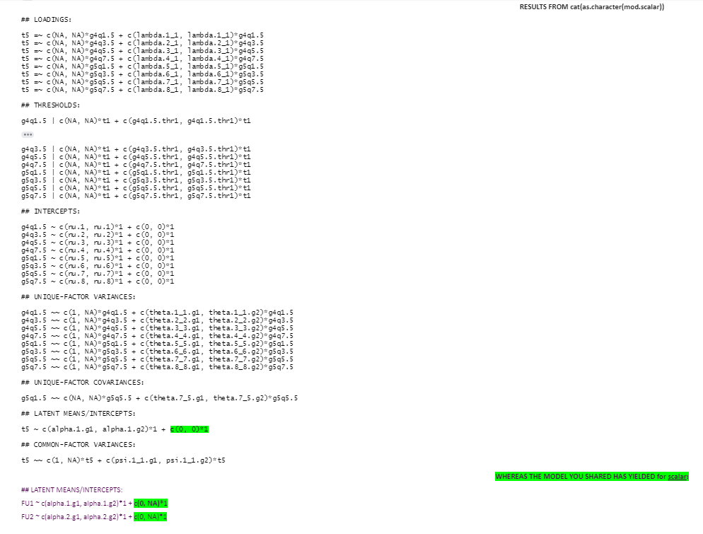
RESULTS FROM cat(as.character(mod.scalar))

## LOADINGS:

t5 =~ c(NA, NA)*g4q1.5 + c(lambda.1_1, lambda.1_1)*g4q1.5

t5 =~ c(NA, NA)*g4q3.5 + c(lambda.2_1, lambda.2_1)*g4q3.5

t5 =~ c(NA, NA)*g4q5.5 + c(lambda.3_1, lambda.3_1)*g4q5.5

t5 =~ c(NA, NA)*g4q7.5 + c(lambda.4_1, lambda.4_1)*g4q7.5

t5 =~ c(NA, NA)*g5q1.5 + c(lambda.5_1, lambda.5_1)*g5q1.5

t5 =~ c(NA, NA)*g5q3.5 + c(lambda.6_1, lambda.6_1)*g5q3.5

t5 =~ c(NA, NA)*g5q5.5 + c(lambda.7_1, lambda.7_1)*g5q5.5

t5 =~ c(NA, NA)*g5q7.5 + c(lambda.8_1, lambda.8_1)*g5q7.5

## THRESHOLDS:

g4q1.5 | c(NA, NA)*t1 + c(g4q1.5.thr1, g4q1.5.thr1)*t1

g4q3.5 | c(NA, NA)*t1 + c(g4q3.5.thr1, g4q3.5.thr1)*t1

g4q5.5 | c(NA, NA)*t1 + c(g4q5.5.thr1, g4q5.5.thr1)*t1

g4q7.5 | c(NA, NA)*t1 + c(g4q7.5.thr1, g4q7.5.thr1)*t1

g5q1.5 | c(NA, NA)*t1 + c(g5q1.5.thr1, g5q1.5.thr1)*t1

g5q3.5 | c(NA, NA)*t1 + c(g5q3.5.thr1, g5q3.5.thr1)*t1

g5q5.5 | c(NA, NA)*t1 + c(g5q5.5.thr1, g5q5.5.thr1)*t1

g5q7.5 | c(NA, NA)*t1 + c(g5q7.5.thr1, g5q7.5.thr1)*t1

## INTERCEPTS:

g4q1.5 ~ c(nu.1, nu.1)*1 + c(0, 0)*1

g4q3.5 ~ c(nu.2, nu.2)*1 + c(0, 0)*1

g4q5.5 ~ c(nu.3, nu.3)*1 + c(0, 0)*1

g4q7.5 ~ c(nu.4, nu.4)*1 + c(0, 0)*1

g5q1.5 ~ c(nu.5, nu.5)*1 + c(0, 0)*1

g5q3.5 ~ c(nu.6, nu.6)*1 + c(0, 0)*1

g5q5.5 ~ c(nu.7, nu.7)*1 + c(0, 0)*1

g5q7.5 ~ c(nu.8, nu.8)*1 + c(0, 0)*1

## UNIQUE-FACTOR VARIANCES:

g4q1.5 ~~ c(1, NA)*g4q1.5 + c(theta.1_1.g1, theta.1_1.g2)*g4q1.5

g4q3.5 ~~ c(1, NA)*g4q3.5 + c(theta.2_2.g1, theta.2_2.g2)*g4q3.5

g4q5.5 ~~ c(1, NA)*g4q5.5 + c(theta.3_3.g1, theta.3_3.g2)*g4q5.5

g4q7.5 ~~ c(1, NA)*g4q7.5 + c(theta.4_4.g1, theta.4_4.g2)*g4q7.5

g5q1.5 ~~ c(1, NA)*g5q1.5 + c(theta.5_5.g1, theta.5_5.g2)*g5q1.5

g5q3.5 ~~ c(1, NA)*g5q3.5 + c(theta.6_6.g1, theta.6_6.g2)*g5q3.5

g5q5.5 ~~ c(1, NA)*g5q5.5 + c(theta.7_7.g1, theta.7_7.g2)*g5q5.5

g5q7.5 ~~ c(1, NA)*g5q7.5 + c(theta.8_8.g1, theta.8_8.g2)*g5q7.5

## UNIQUE-FACTOR COVARIANCES:

g5q1.5 ~~ c(NA, NA)*g5q5.5 + c(theta.7_5.g1, theta.7_5.g2)*g5q5.5

## LATENT MEANS/INTERCEPTS:

t5 ~ c(alpha.1.g1, alpha.1.g2)*1 + c(0, 0)*1

## COMMON-FACTOR VARIANCES:

t5 ~~ c(1, NA)*t5 + c(psi.1_1.g1, psi.1_1.g2)*t5

WHEREAS THE MODEL YOU SHARED HAS YIELDED for scalar:

## LATENT MEANS/INTERCEPTS:

FU1 ~ c(alpha.1.g1, alpha.1.g2)*1 + c(0, NA)*1

FU2 ~ c(alpha.2.g1, alpha.2.g2)*1 + c(0, NA)*1

 

[Terrence Jorgensen]

RESULTS FROM cat(as.character(mod.scalar))

## LOADINGS:

t5 =~ c(NA, NA)*g4q1.5 + c(lambda.1_1, lambda.1_1)*g4q1.5

t5 =~ c(NA, NA)*g4q3.5 + c(lambda.2_1, lambda.2_1)*g4q3.5

t5 =~ c(NA, NA)*g4q5.5 + c(lambda.3_1, lambda.3_1)*g4q5.5

t5 =~ c(NA, NA)*g4q7.5 + c(lambda.4_1, lambda.4_1)*g4q7.5

t5 =~ c(NA, NA)*g5q1.5 + c(lambda.5_1, lambda.5_1)*g5q1.5

t5 =~ c(NA, NA)*g5q3.5 + c(lambda.6_1, lambda.6_1)*g5q3.5

t5 =~ c(NA, NA)*g5q5.5 + c(lambda.7_1, lambda.7_1)*g5q5.5

t5 =~ c(NA, NA)*g5q7.5 + c(lambda.8_1, lambda.8_1)*g5q7.5

## THRESHOLDS:

<span style="font-family:"Lucida Console";color:black;border:1pt none windowte

The output you posted cut off here.  Could you just post the scalar syntax for me to see?

[Pavneet Bharaj]

Good Evening Dr. Terrence.

I hope this works. I am pasting the syntax as well as the output. I highlighted the o output in green to show the difference in results between the model that you stated above and the model that I have specified. 

type5 <- 't5=~ g4q1.5+ g4q3.5+ g4q5.5 + g4q7.5 + g5q1.5+ g5q3.5+ g5q5.5 + g5q7.5 

g5q1.5 ~~ g5q5.5'

 

fit.type5<- cfa(model=type5, data=data, group="group", parameterization="theta", estimator="wlsmv", meanstructure=T, std.lv=T, ordered=c("g4q1.5", "g4q3.5", "g4q5.5", "g4q7.5", "g5q1.5", "g5q3.5", "g5q5.5", "g5q7.5"))

summary(fit.type5, standardized=T , rsquare=T, fit.measures=T)

 

#---- using measEqsynatx( ) --------#

mod.configural<-measEq.syntax(fit.type5, group="group")

mod.scalar<-measEq.syntax(fit.type5, group.equal=c("thresholds","loadings","intercepts"))

cat(as.character(mod.configural))

cat(as.character(mod.scalar))

 

RESULTS FROM cat(as.character(mod.configural))

> cat(as.character(mod.configural))

## LOADINGS:

 

t5 =~ c(NA, NA)*g4q1.5 + c(lambda.1_1.g1, lambda.1_1.g2)*g4q1.5

RESULTS FROM cat(as.character(mod.scalar))

## LOADINGS:

t5 =~ c(NA, NA)*g4q1.5 + c(lambda.1_1, lambda.1_1)*g4q1.5

t5 =~ c(NA, NA)*g4q3.5 + c(lambda.2_1, lambda.2_1)*g4q3.5

t5 =~ c(NA, NA)*g4q5.5 + c(lambda.3_1, lambda.3_1)*g4q5.5

t5 =~ c(NA, NA)*g4q7.5 + c(lambda.4_1, lambda.4_1)*g4q7.5

t5 =~ c(NA, NA)*g5q1.5 + c(lambda.5_1, lambda.5_1)*g5q1.5

t5 =~ c(NA, NA)*g5q3.5 + c(lambda.6_1, lambda.6_1)*g5q3.5

t5 =~ c(NA, NA)*g5q5.5 + c(lambda.7_1, lambda.7_1)*g5q5.5

t5 =~ c(NA, NA)*g5q7.5 + c(lambda.8_1, lambda.8_1)*g5q7.5

## THRESHOLDS:

g4q1.5 | c(NA, NA)*t1 + c(g4q1.5.thr1, g4q1.5.thr1)*t1

[Pavneet Bharaj]

I am also attaching a screenshot of the output of "scalar" model.

[Terrence Jorgensen]

I am also attaching a screenshot of the output of "scalar" model.

My example had 2 factors, whereas you have 1.  So I tried running my example with only 1 factor, and I saw the same problem you found.  Thanks for helping me track this down.  It is now fixed in the development version (0.5-1.908), which you can download with the same syntax as before.

devtools::install_github("simsem/semTools/semTools")

[Pavneet Bharaj]

Good Evening Dr. Terrence.

Thanks a lot for your help on this.

I worked on all of my models and it worked perfectly. I really appreciate your help.

Regards,

Pavneet Kaur

[Pavneet Bharaj]

Good Evening Dr. Terrence.

I am working on checking the partial invariance of the model:

type4 <- 'type4=~ g4q1.4+ g4q3.4+ g4q5.4 + g4q7.4 + g5q1.4+ g5q3.4+ g5q5.4 + g5q7.4 

        g5q1.4 ~~ g5q7.4'

 

So, in this model I tried to assess for which item I need to freely estimate the factor loadings to attain the invariance at loadings, threshold, and intercepts level (Since my data is binary).

For some of the items, when I freely estimated the loadings for both groups, I got results as:

test_partial_1<-measEq.syntax(type4, data=data,  ID.cat="Wu.Estabrook.2016", group="group", group.equal=c("thresholds","loadings","intercepts"),   group.partial=c("type4=~g4q1.4"),warn=T, return.fit=T, parameterization="theta", estimator="wlsmv",  meanstructure=TRUE,std.lv=T,                          ordered=c("g4q1.4", "g4q3.4", "g4q5.4", "g4q7.4", "g5q1.4", "g5q3.4", "g5q5.4", "g5q7.4"))

> summary(test_partial_1, fit.measures=T, rsquare=T)

lavaan 0.6-3 ended normally after 176 iterations

 

  Optimization method                           NLMINB

  Number of free parameters                         44

  Number of equality constraints                    15

 

  Number of observations per group        

  0                                                919

  1                                                926

 

  Estimator                                       DWLS      Robust

  Model Fit Test Statistic                      58.451      64.028

  Degrees of freedom                                43          43

  P-value (Chi-square)                           0.058       0.020

  Scaling correction factor                                  0.911

  Shift parameter for each group:

    0                                                       -0.063

    1                                                       -0.064

    for simple second-order correction (Mplus variant)

 

Chi-square for each group:

 

  0                                             29.154      31.936

  1                                             29.297      32.092

 

Model test baseline model:

 

  Minimum Function Test Statistic              312.409     302.732

  Degrees of freedom                                56          56

  P-value                                        0.000       0.000

 

User model versus baseline model:

 

  Comparative Fit Index (CFI)                    0.940       0.915

  Tucker-Lewis Index (TLI)                       0.922       0.889

 

  Robust Comparative Fit Index (CFI)                            NA

  Robust Tucker-Lewis Index (TLI)                               NA

 

Root Mean Square Error of Approximation:

 

  RMSEA                                          0.020       0.023

  90 Percent Confidence Interval          0.000  0.032       0.009  0.034

  P-value RMSEA <= 0.05                          1.000       1.000

 

  Robust RMSEA                                                  NA

  90 Percent Confidence Interval                                NA     NA

 

Standardized Root Mean Square Residual:

 

  SRMR                                           0.043       0.043

 

Parameter Estimates:

 

  Information                                 Expected

  Information saturated (h1) model        Unstructured

  Standard Errors                           Robust.sem

 

 

Group 1 [0]:

 

Latent Variables:

                   Estimate  Std.Err  z-value  P(>|z|)

  type4 =~                                           

    g4q1.4  (l.1_)    0.152    0.069    2.212    0.027

    g4q3.4  (l.2_)    0.362    0.072    5.029    0.000

    g4q5.4  (l.3_)    0.519    0.099    5.269    0.000

    g4q7.4  (l.4_)    0.435    0.079    5.529    0.000

    g5q1.4  (l.5_)    0.601    0.109    5.528    0.000

    g5q3.4  (l.6_)    0.345    0.079    4.363    0.000

    g5q5.4  (l.7_)    0.294    0.074    3.974    0.000

    g5q7.4  (l.8_)   -0.024    0.024   -1.014    0.311

 

Covariances:

                   Estimate  Std.Err  z-value  P(>|z|)

 .g5q1.4 ~~                                          

   .g5q7.4  (t.8_)   -0.248    0.061   -4.070    0.000

 

Intercepts:

                   Estimate  Std.Err  z-value  P(>|z|)

   .g4q1.4  (nu.1)    0.000                          

   .g4q3.4  (nu.2)    0.000                          

   .g4q5.4  (nu.3)    0.000                          

   .g4q7.4  (nu.4)    0.000                          

   .g5q1.4  (nu.5)    0.000                           

   .g5q3.4  (nu.6)    0.000                          

   .g5q5.4  (nu.7)    0.000                          

   .g5q7.4  (nu.8)    0.000                          

    type4   (a.1.)    0.000                          

 

Thresholds:

                   Estimate  Std.Err  z-value  P(>|z|)

    g41.4|1 (g41.)   -0.413    0.043   -9.537    0.000

    g43.4|1 (g43.)   -0.979    0.056  -17.524    0.000

    g45.4|1 (g45.)    0.015    0.046    0.322    0.747

    g47.4|1 (g47.)   -0.562    0.050  -11.291    0.000

    g51.4|1 (g51.)   -0.248    0.049   -5.072    0.000

    g53.4|1 (g53.)    0.130    0.043    3.049    0.002

    g55.4|1 (g55.)   -0.105    0.041   -2.559    0.011

    g57.4|1 (g57.)    0.379    0.042    8.917    0.000

 

Variances:

                   Estimate  Std.Err  z-value  P(>|z|)

   .g4q1.4  (t.1_)    1.000                          

   .g4q3.4  (t.2_)    1.000                          

   .g4q5.4  (t.3_)    1.000                          

   .g4q7.4  (t.4_)    1.000                           

   .g5q1.4  (t.5_)    1.000                          

   .g5q3.4  (t.6_)    1.000                          

   .g5q5.4  (t.7_)    1.000                          

   .g5q7.4  (t.8_)    1.000                          

    type4   (p.1_)    1.000                          

 

Scales y*:

                   Estimate  Std.Err  z-value  P(>|z|)

    g4q1.4            0.989                          

    g4q3.4            0.940                          

    g4q5.4            0.888                           

    g4q7.4            0.917                          

    g5q1.4            0.857                          

    g5q3.4            0.945                          

    g5q5.4            0.959                          

    g5q7.4            1.000                          

 

R-Square:

                   Estimate

    g4q1.4            0.023

    g4q3.4            0.116

    g4q5.4            0.212

    g4q7.4            0.159

    g5q1.4            0.266

    g5q3.4            0.106

    g5q5.4            0.080

    g5q7.4            0.001

 

 

Group 2 [1]:

 

Latent Variables:

                   Estimate  Std.Err  z-value  P(>|z|)

  type4 =~                                           

    g4q1.4  (l.1_)    0.059    0.063    0.941    0.347

    g4q3.4  (l.2_)    0.362    0.072    5.029    0.000

    g4q5.4  (l.3_)    0.519    0.099    5.269    0.000

    g4q7.4  (l.4_)    0.435    0.079    5.529    0.000

    g5q1.4  (l.5_)    0.601    0.109    5.528    0.000

    g5q3.4  (l.6_)    0.345    0.079    4.363    0.000

    g5q5.4  (l.7_)    0.294    0.074    3.974    0.000

    g5q7.4  (l.8_)   -0.024    0.024   -1.014    0.311

 

Covariances:

                   Estimate  Std.Err  z-value  P(>|z|)

 .g5q1.4 ~~                                          

   .g5q7.4  (t.8_)   -0.197    0.112   -1.764    0.078

 

Intercepts:

                   Estimate  Std.Err  z-value  P(>|z|)

   .g4q1.4  (nu.1)    0.000                          

   .g4q3.4  (nu.2)    0.000                          

   .g4q5.4  (nu.3)    0.000                           

   .g4q7.4  (nu.4)    0.000                          

   .g5q1.4  (nu.5)    0.000                          

   .g5q3.4  (nu.6)    0.000                          

   .g5q5.4  (nu.7)    0.000                          

   .g5q7.4  (nu.8)    0.000                          

    type4   (a.1.)    0.473    0.242    1.960    0.050

 

Thresholds:

                   Estimate  Std.Err  z-value  P(>|z|)

    g41.4|1 (g41.)   -0.413    0.043   -9.537    0.000

    g43.4|1 (g43.)   -0.979    0.056  -17.524    0.000

    g45.4|1 (g45.)    0.015    0.046    0.322    0.747

    g47.4|1 (g47.)   -0.562    0.050  -11.291    0.000

    g51.4|1 (g51.)   -0.248    0.049   -5.072    0.000

    g53.4|1 (g53.)    0.130    0.043    3.049    0.002

    g55.4|1 (g55.)   -0.105    0.041   -2.559    0.011

    g57.4|1 (g57.)    0.379    0.042    8.917    0.000

 

Variances:

                   Estimate  Std.Err  z-value  P(>|z|)

   .g4q1.4  (t.1_)    2.324    0.921    2.523    0.012

   .g4q3.4  (t.2_)    1.158    0.236    4.902    0.000

   .g4q5.4  (t.3_)   18.140   15.517    1.169    0.242

   .g4q7.4  (t.4_)    1.612    0.580    2.781    0.005

   .g5q1.4  (t.5_)    6.015    3.908    1.539    0.124

   .g5q3.4  (t.6_)    4.381    3.515    1.246    0.213

   .g5q5.4  (t.7_)    4.253    3.381    1.258    0.209

   .g5q7.4  (t.8_)    0.320    0.085    3.761    0.000

    type4   (p.1_)    3.402    1.379    2.467    0.014

 

Scales y*:

                   Estimate  Std.Err  z-value  P(>|z|)

    g4q1.4            0.654                           

    g4q3.4            0.790                          

    g4q5.4            0.229                          

    g4q7.4            0.666                          

    g5q1.4            0.372                          

    g5q3.4            0.457                          

    g5q5.4            0.469                          

    g5q7.4            1.762                          

 

R-Square:

                   Estimate

    g4q1.4            0.005

    g4q3.4            0.278

    g4q5.4            0.048

    g4q7.4            0.285

    g5q1.4            0.170

    g5q3.4            0.085

    g5q5.4            0.065

    g5q7.4            0.006

 

But, when I tried to use the same code for some other items (within above model), I got this message:

test_partial_3<-measEq.syntax(type4, data=data,  ID.cat="Wu.Estabrook.2016",  group="group", group.equal=c("thresholds","loadings","intercepts"), parameterization="theta", estimator="wlsmv",meanstructure=TRUE, std.lv=T,   group.partial=c("type4=~g4q5.4"),warn=T, return.fit=T,  ordered=c("g4q1.4", "g4q3.4", "g4q5.4", "g4q7.4",   "g5q1.4", "g5q3.4", "g5q5.4", "g5q7.4"))

 

Warning messages:

1: In lav_model_vcov(lavmodel = lavmodel, lavsamplestats = lavsamplestats,  :

  lavaan WARNING:

    The variance-covariance matrix of the estimated parameters (vcov)

    does not appear to be positive definite! The smallest eigenvalue

    (= 2.197847e-14) is close to zero. This may be a symptom that the

    model is not identified.

2: In lavaan::lavaan(model = "## LOADINGS:\n\ntype4 =~ c(NA, NA)*g4q1.4 + c(lambda.1_1, lambda.1_1)*g4q1.4\ntype4 =~ c(NA, NA)*g4q3.4 + c(lambda.2_1, lambda.2_1)*g4q3.4\ntype4 =~ c(NA, NA)*g4q5.4 + c(lambda.3_1.g1, lambda.3_1.g2)*g4q5.4\ntype4 =~ c(NA, NA)*g4q7.4 + c(lambda.4_1, lambda.4_1)*g4q7.4\ntype4 =~ c(NA, NA)*g5q1.4 + c(lambda.5_1, lambda.5_1)*g5q1.4\ntype4 =~ c(NA, NA)*g5q3.4 + c(lambda.6_1, lambda.6_1)*g5q3.4\ntype4 =~ c(NA, NA)*g5q5.4 + c(lambda.7_1, lambda.7_1)*g5q5.4\ntype4 =~ c(NA, NA)*g5q7.4 + c(lambda.8_1, lambda.8_1)*g5q7.4\n\n## THRESHOLDS:\n\ng4q1.4 | c(NA, NA)*t1 + c(g4q1.4.thr1, g4q1.4.thr1)*t1\ng4q3.4 | c(NA, NA)*t1 + c(g4q3.4.thr1, g4q3.4.thr1)*t1\ng4q5.4 | c(NA, NA)*t1 + c(g4q5.4.thr1, g4q5.4.thr1)*t1\ng4q7.4 | c(NA, NA)*t1 + c(g4q7.4.thr1, g4q7.4.thr1)*t1\ng5q1.4 | c(NA, NA)*t1 + c(g5q1.4.thr1, g5q1.4.thr1)*t1\ng5q3.4 | c(NA, NA)*t1 + c(g5q3.4.thr1, g5q3.4.thr1)*t1\ng5q5.4 | c(NA, NA)*t1 + c(g5q5.4.thr1, g5q5.4.thr1)*t1\ng5q7.4 | c(NA, NA)*t1 + c(g5q7.4.thr1, g5q7.4.thr1)*t1\n\n## INTERCEPTS:\n\ng4q1.4 ~ c(nu.1, nu.1)*1 + c(0, 0)*1\ng4q3.4 ~ c(nu.2, nu.2)*1 + c(0, 0)*1\ng4q5.4 ~ c(nu.3, nu.3)*1 + c(0, 0)*1\ng4q7.4 ~ c(nu.4, nu.4)*1 + c(0, 0)*1\ng5q1.4 ~ c(nu.5, nu.5)*1 + c(0, 0)*1\ng5q3.4 ~ c(nu.6, nu.6)*1 + c(0, 0)*1\ng5q5.4 ~ c(nu.7, nu.7)*1 + c(0, 0)*1\ng5q7.4 ~ c(nu.8, nu.8)*1 + c(0, 0)*1\n\n## UNIQUE-FACTOR VARIANCES:\n\ng4q1.4 ~~ c(1, NA)*g4q1.4 + c(theta.1_1.g1, theta.1_1.g2)*g4q1.4\ng4q3.4 ~~ c(1, NA)*g4q3.4 + c(theta.2_2.g1, theta.2_2.g2)*g4q3.4\ng4q5.4 ~~ c(1, NA)*g4q5.4 + c(theta.3_3.g1, theta.3_3.g2)*g4q5.4\ng4q7.4 ~~ c(1, NA)*g4q7.4 + c(theta.4_4.g1, theta.4_4.g2)*g4q7.4\ng5q1.4 ~~ c(1, NA)*g5q1.4 + c(theta.5_5.g1, theta.5_5.g2)*g5q1.4\ng5q3.4 ~~ c(1, NA)*g5q3.4 + c(theta.6_6.g1, theta.6_6.g2)*g5q3.4\ng5q5.4 ~~ c(1, NA)*g5q5.4 + c(theta.7_7.g1, theta.7_7.g2)*g5q5.4\ng5q7.4 ~~ c(1, NA)*g5q7.4 + c(theta.8_8.g1, theta.8_8.g2)*g5q7.4\n\n## UNIQUE-FACTOR COVARIANCES:\n\ng5q1.4 ~~ c(NA, NA)*g5q7.4 + c(theta.8_5.g1, theta.8_5.g2)*g5q7.4\n\n## LATENT MEANS/INTERCEPTS:\n\ntype4 ~ c(alpha.1.g1, alpha.1.g2)*1 + c(0, NA)*1\n\n## COMMON-FACTOR VARIANCES:\n\ntype4 ~~ c(1, NA)*type4 + c(psi.1_1.g1, psi.1_1.g2)*type4\n",  :

  lavaan WARNING: not all elements of the gradient are (near) zero;

                  the optimizer may not have found a local solution;

                  use lavInspect(fit, "optim.gradient") to investigate

 

  

I tried to run the same model by also freely estimating the threshold for that particular item for both groups and  I got the results:

> # ================== third item ============== #

> test_partial_3<-measEq.syntax(type4, data=data,  ID.cat="Wu.Estabrook.2016",group="group", group.equal=c("thresholds","loadings","intercepts"),

group.partial=c("type4=~g4q5.4", "g4q5.4|t1"),warn=T, return.fit=T, ordered=c("g4q1.4", "g4q3.4", "g4q5.4", "g4q7.4", "g5q1.4", "g5q3.4", "g5q5.4", "g5q7.4"),parameterization="theta", estimator="wlsmv", meanstructure=TRUE, std.lv=T )

> summary(test_partial_3, fit.measures=T, rsquare=T)

lavaan 0.6-3 ended normally after 159 iterations

  Optimization method                           NLMINB

  Number of free parameters                         43

  Number of equality constraints                    14

  Number of observations per group         

  0                                                919

  1                                                926

  Estimator                                       DWLS      Robust

  Model Fit Test Statistic                      57.106      62.068

  Degrees of freedom                                43          43

  P-value (Chi-square)                           0.073       0.030

  Scaling correction factor                                  0.914

  Shift parameter for each group:

    0                                                       -0.193

    1                                                       -0.194

    for simple second-order correction (Mplus variant)

Chi-square for each group:

  0                                             28.977      31.498

  1                                             28.129      30.569

Model test baseline model:

  Minimum Function Test Statistic              312.409     302.732

  Degrees of freedom                                56          56

  P-value                                        0.000       0.000

User model versus baseline model:

  Comparative Fit Index (CFI)                    0.945       0.923

  Tucker-Lewis Index (TLI)                       0.928       0.899

  Robust Comparative Fit Index (CFI)                            NA

  Robust Tucker-Lewis Index (TLI)                               NA

Root Mean Square Error of Approximation:

  RMSEA                                          0.019       0.022

  90 Percent Confidence Interval          0.000  0.031       0.007  0.033

  P-value RMSEA <= 0.05                          1.000       1.000

  Robust RMSEA                                                  NA

  90 Percent Confidence Interval                                NA     NA

Standardized Root Mean Square Residual:

  SRMR                                           0.043       0.043

Parameter Estimates:

  Information                                 Expected

  Information saturated (h1) model        Unstructured

  Standard Errors                           Robust.sem

Group 1 [0]:

Latent Variables:

                   Estimate  Std.Err  z-value  P(>|z|)

  type4 =~                                            

    g4q1.4  (l.1_)    0.107    0.051    2.097    0.036

    g4q3.4  (l.2_)    0.369    0.073    5.025    0.000

    g4q5.4  (l.3_)    0.514    0.098    5.275    0.000

    g4q7.4  (l.4_)    0.452    0.082    5.526    0.000

    g5q1.4  (l.5_)    0.606    0.110    5.494    0.000

    g5q3.4  (l.6_)    0.346    0.079    4.384    0.000

    g5q5.4  (l.7_)    0.291    0.074    3.917    0.000

    g5q7.4  (l.8_)   -0.024    0.024   -1.003    0.316

Covariances:

                   Estimate  Std.Err  z-value  P(>|z|)

 .g5q1.4 ~~                                           

   .g5q7.4  (t.8_)   -0.249    0.061   -4.072    0.000

Intercepts:

                   Estimate  Std.Err  z-value  P(>|z|)

   .g4q1.4  (nu.1)    0.000                           

   .g4q3.4  (nu.2)    0.000                           

   .g4q5.4  (nu.3)    0.000                           

   .g4q7.4  (nu.4)    0.000                           

   .g5q1.4  (nu.5)    0.000                           

   .g5q3.4  (nu.6)    0.000                           

   .g5q5.4  (nu.7)    0.000                           

   .g5q7.4  (nu.8)    0.000                           

    type4   (a.1.)    0.000                           

Thresholds:

                   Estimate  Std.Err  z-value  P(>|z|)

    g41.4|1 (g41.)   -0.417    0.043   -9.723    0.000

    g43.4|1 (g43.)   -0.980    0.056  -17.424    0.000

    g45.4|1 (g45.)   -0.002    0.047   -0.033    0.974

    g47.4|1 (g47.)   -0.562    0.050  -11.161    0.000

    g51.4|1 (g51.)   -0.244    0.049   -4.955    0.000

    g53.4|1 (g53.)    0.141    0.043    3.257    0.001

    g55.4|1 (g55.)   -0.102    0.041   -2.472    0.013

    g57.4|1 (g57.)    0.379    0.042    8.919    0.000

Variances:

                   Estimate  Std.Err  z-value  P(>|z|)

   .g4q1.4  (t.1_)    1.000                           

   .g4q3.4  (t.2_)    1.000                           

   .g4q5.4  (t.3_)    1.000                           

   .g4q7.4  (t.4_)    1.000                           

   .g5q1.4  (t.5_)    1.000                           

   .g5q3.4  (t.6_)    1.000                           

   .g5q5.4  (t.7_)    1.000                           

   .g5q7.4  (t.8_)    1.000                           

    type4   (p.1_)    1.000                           

Scales y*:

                   Estimate  Std.Err  z-value  P(>|z|)

    g4q1.4            0.994                           

    g4q3.4            0.938                           

    g4q5.4            0.889                           

    g4q7.4            0.911                           

    g5q1.4            0.855                           

    g5q3.4            0.945                           

    g5q5.4            0.960                           

    g5q7.4            1.000                           

R-Square:

                   Estimate

    g4q1.4            0.011

    g4q3.4            0.120

    g4q5.4            0.209

    g4q7.4            0.170

    g5q1.4            0.268

    g5q3.4            0.107

    g5q5.4            0.078

    g5q7.4            0.001

Group 2 [1]:

Latent Variables:

                   Estimate  Std.Err  z-value  P(>|z|)

  type4 =~                                            

    g4q1.4  (l.1_)    0.107    0.051    2.097    0.036

    g4q3.4  (l.2_)    0.369    0.073    5.025    0.000

    g4q5.4  (l.3_)    0.134    0.048    2.779    0.005

    g4q7.4  (l.4_)    0.452    0.082    5.526    0.000

    g5q1.4  (l.5_)    0.606    0.110    5.494    0.000

    g5q3.4  (l.6_)    0.346    0.079    4.384    0.000

    g5q5.4  (l.7_)    0.291    0.074    3.917    0.000

    g5q7.4  (l.8_)   -0.024    0.024   -1.003    0.316

Covariances:

                   Estimate  Std.Err  z-value  P(>|z|)

 .g5q1.4 ~~                                           

   .g5q7.4  (t.8_)   -0.222    0.126   -1.765    0.078

Intercepts:

                   Estimate  Std.Err  z-value  P(>|z|)

   .g4q1.4  (nu.1)    0.000                           

   .g4q3.4  (nu.2)    0.000                           

   .g4q5.4  (nu.3)    0.000                           

   .g4q7.4  (nu.4)    0.000                           

   .g5q1.4  (nu.5)    0.000                           

   .g5q3.4  (nu.6)    0.000                           

   .g5q5.4  (nu.7)    0.000                           

   .g5q7.4  (nu.8)    0.000                           

    type4   (a.1.)    0.625    0.303    2.064    0.039

Thresholds:

                   Estimate  Std.Err  z-value  P(>|z|)

    g41.4|1 (g41.)   -0.417    0.043   -9.723    0.000

    g43.4|1 (g43.)   -0.980    0.056  -17.424    0.000

    g45.4|1 (g45.)    0.087    0.055    1.564    0.118

    g47.4|1 (g47.)   -0.562    0.050  -11.161    0.000

    g51.4|1 (g51.)   -0.244    0.049   -4.955    0.000

    g53.4|1 (g53.)    0.141    0.043    3.257    0.001

    g55.4|1 (g55.)   -0.102    0.041   -2.472    0.013

    g57.4|1 (g57.)    0.379    0.042    8.919    0.000

Variances:

                   Estimate  Std.Err  z-value  P(>|z|)

   .g4q1.4  (t.1_)    2.989    1.240    2.410    0.016

   .g4q3.4  (t.2_)    1.278    0.282    4.527    0.000

   .g4q5.4  (t.3_)    1.000                           

   .g4q7.4  (t.4_)    1.945    0.784    2.480    0.013

   .g5q1.4  (t.5_)    7.431    5.059    1.469    0.142

   .g5q3.4  (t.6_)    4.770    4.025    1.185    0.236

   .g5q5.4  (t.7_)    4.889    4.002    1.222    0.222

   .g5q7.4  (t.8_)    0.326    0.088    3.711    0.000

    type4   (p.1_)    3.647    1.567    2.328    0.020

Scales y*:

                   Estimate  Std.Err  z-value  P(>|z|)

    g4q1.4            0.574                           

    g4q3.4            0.751                           

    g4q5.4            0.969                           

    g4q7.4            0.610                           

    g5q1.4            0.338                           

    g5q3.4            0.438                           

    g5q5.4            0.439                           

    g5q7.4            1.747                           

R-Square:

                   Estimate

    g4q1.4            0.014

    g4q3.4            0.280

    g4q5.4            0.062

    g4q7.4            0.277

    g5q1.4            0.153

    g5q3.4            0.084

    g5q5.4            0.059

    g5q7.4            0.006

 

 

Based on the and notes https://crmda.dept.ku.edu/guides/21.LavaanSyntaxGuide/21.LavaanSyntaxGuide.pdf  on lavaan I found at “The loadings and thresholds are both constrained to equality across groups “g”, allowing the scale of the ordinal indicators to be freely estimated in the second group” which I agree with, but I am thinking won’t freely estimating the thresholds for two groups will impact the degrees of freedom?

As in both the specifications (where I just freely estimated the loadings for the item g4q1.4 and where I freely estimated the loading as well as the threshold for item g4q5.4), the scaled degrees of freedom is 43.

I am curious if the scaled degrees of freedom don’t take in account the estimated values of the thresholds? Because the number of freely estimated and equal parameters are different in both the models (highlighted in green color).

Thanks in advance.

Regards,

Pavneet Kaur

[Terrence Jorgensen]

Again, your output was cut off.  Please only paste the parts that are necessary to answer your question.

[Pavneet Bharaj]

Good evening Dr. Terrence. Sorry for the output.  I wasn’t sure which parameter value would you require, so here I deleted some of the information in output that I felt might be unnecessary for my concern. I am working on checking the partial invariance of the model:

type4 <- 'type4=~ g4q1.4+ g4q3.4+ g4q5.4 + g4q7.4 + g5q1.4+ g5q3.4+ g5q5.4 + g5q7.4 

        g5q1.4 ~~ g5q7.4'

 So, in this model I tried to assess for which item I need to freely estimate the factor loadings to attain the invariance at loadings, threshold, and intercepts level (Since my data is binary). For some of the items, when I freely estimated the loadings for both groups, I got results as:

test_partial_1<-measEq.syntax(type4, data=data,  ID.cat="Wu.Estabrook.2016", group="group", group.equal = c("thresholds","loadings","intercepts"),   group.partial = c("type4=~g4q1.4"), warn=T, return.fit=T, parameterization="theta", estimator="wlsmv",  meanstructure=TRUE,std.lv=T, ordered=c("g4q1.4", "g4q3.4", "g4q5.4", "g4q7.4", "g5q1.4", "g5q3.4", "g5q5.4", "g5q7.4"))

 Group 1 [0]:

 Latent Variables:

                   Estimate  Std.Err  z-value  P(>|z|)

  type4 =~                                           

    g4q1.4  (l.1_)    0.152    0.069    2.212    0.027

    g4q3.4  (l.2_)    0.362    0.072    5.029    0.000

    g4q5.4  (l.3_)    0.519    0.099    5.269    0.000

    g4q7.4  (l.4_)    0.435    0.079    5.529    0.000

    g5q1.4  (l.5_)    0.601    0.109    5.528    0.000

    g5q3.4  (l.6_)    0.345    0.079    4.363    0.000

    g5q5.4  (l.7_)    0.294    0.074    3.974    0.000

    g5q7.4  (l.8_)   -0.024    0.024   -1.014    0.311

 Covariances:

                   Estimate  Std.Err  z-value  P(>|z|)

 .g5q1.4 ~~   .g5q7.4  (t.8_)   -0.248    0.061   -4.070    0.000

 Intercepts:

                  (all set to zero)

 Thresholds:

                   Estimate  Std.Err  z-value  P(>|z|)

    g41.4|1 (g41.)   -0.413    0.043   -9.537    0.000

    g43.4|1 (g43.)   -0.979    0.056  -17.524    0.000

    g45.4|1 (g45.)    0.015    0.046    0.322    0.747

    g47.4|1 (g47.)   -0.562    0.050  -11.291    0.000

    g51.4|1 (g51.)   -0.248    0.049   -5.072    0.000

    g53.4|1 (g53.)    0.130    0.043    3.049    0.002

    g55.4|1 (g55.)   -0.105    0.041   -2.559    0.011

    g57.4|1 (g57.)    0.379    0.042    8.917    0.000

 Variances:

(all set to 1)

 Group 2 [1]:

 Latent Variables:

                   Estimate  Std.Err  z-value  P(>|z|)

  type4 =~                                           

    g4q1.4  (l.1_)    0.059    0.063    0.941    0.347

    g4q3.4  (l.2_)    0.362    0.072    5.029    0.000

    g4q5.4  (l.3_)    0.519    0.099    5.269    0.000

    g4q7.4  (l.4_)    0.435    0.079    5.529    0.000

    g5q1.4  (l.5_)    0.601    0.109    5.528    0.000

    g5q3.4  (l.6_)    0.345    0.079    4.363    0.000

    g5q5.4  (l.7_)    0.294    0.074    3.974    0.000

    g5q7.4  (l.8_)   -0.024    0.024   -1.014    0.311

 Covariances:

                   Estimate  Std.Err  z-value  P(>|z|)

 .g5q1.4 ~~   .g5q7.4  (t.8_)   -0.197    0.112   -1.764    0.078

 Intercepts:

                   Estimate  Std.Err  z-value  P(>|z|)

   .(intercepts of items are all 0)

    type4   (a.1.)    0.473    0.242    1.960    0.050

 

Thresholds:

                   Estimate  Std.Err  z-value  P(>|z|)

    g41.4|1 (g41.)   -0.413    0.043   -9.537    0.000

    g43.4|1 (g43.)   -0.979    0.056  -17.524    0.000

    g45.4|1 (g45.)    0.015    0.046    0.322    0.747

    g47.4|1 (g47.)   -0.562    0.050  -11.291    0.000

    g51.4|1 (g51.)   -0.248    0.049   -5.072    0.000

    g53.4|1 (g53.)    0.130    0.043    3.049    0.002

    g55.4|1 (g55.)   -0.105    0.041   -2.559    0.011

    g57.4|1 (g57.)    0.379    0.042    8.917    0.000

 

Variances:

                   Estimate  Std.Err  z-value  P(>|z|)

   .g4q1.4  (t.1_)    2.324    0.921    2.523    0.012

   .g4q3.4  (t.2_)    1.158    0.236    4.902    0.000

   .g4q5.4  (t.3_)   18.140   15.517    1.169    0.242

   .g4q7.4  (t.4_)    1.612    0.580    2.781    0.005

   .g5q1.4  (t.5_)    6.015    3.908    1.539    0.124

   .g5q3.4  (t.6_)    4.381    3.515    1.246    0.213

   .g5q5.4  (t.7_)    4.253    3.381    1.258    0.209

   .g5q7.4  (t.8_)    0.320    0.085    3.761    0.000

    type4   (p.1_)    3.402    1.379    2.467    0.014

 

But, when I tried to use the same code for some other items (within above model), I got this message:

test_partial_3<-measEq.syntax(type4, data=data,  ID.cat="Wu.Estabrook.2016",  group="group", parameterization="theta", group.equal = c("thresholds","loadings","intercepts"), estimator="wlsmv", meanstructure= TRUE, std.lv=T,   group.partial=c("type4=~g4q5.4"),warn=T, return.fit=T,  ordered=c("g4q1.4", "g4q3.4", "g4q5.4", "g4q7.4",   "g5q1.4", "g5q3.4", "g5q5.4", "g5q7.4"))

 Warning messages:

1: In lav_model_vcov(lavmodel = lavmodel, lavsamplestats = lavsamplestats,  :  lavaan WARNING:    The variance-covariance matrix of the estimated parameters (vcov)

    does not appear to be positive definite! The smallest eigenvalue    (= 2.197847e-14) is close to zero. This may be a symptom that the    model is not identified.

2: In lavaan::lavaan(model = "## LOADINGS:\n\ntype4 =~ c(NA, NA)*g4q1.4 + c(lambda.1_1, lambda.1_1)*g4q1.4\ntype4 =~ c(NA, NA)*g4q3.4 + c(lambda.2_1, lambda.2_1)*g4q3.4\ntype4 =~ c(NA, NA)*g4q5.4 + c(lambda.3_1.g1, lambda.3_1.g2)*g4q5.4\ntype4 =~ c(NA, NA)*g4q7.4 + c(lambda.4_1, lambda.4_1)*g4q7.4\ntype4 =~ c(NA, NA)*g5q1.4 + c(lambda.5_1, lambda.5_1)*g5q1.4\ntype4 =~ c(NA, NA)*g5q3.4 + c(lambda.6_1, lambda.6_1)*g5q3.4\ntype4 =~ c(NA, NA)*g5q5.4 + c(lambda.7_1, lambda.7_1)*g5q5.4\ntype4 =~ c(NA, NA)*g5q7.4 + c(lambda.8_1, lambda.8_1)*g5q7.4\n\n## THRESHOLDS:\n\ng4q1.4 | c(NA, NA)*t1 + c(g4q1.4.thr1, g4q1.4.thr1)*t1\ng4q3.4 | c(NA, NA)*t1 + c(g4q3.4.thr1, g4q3.4.thr1)*t1\ng4q5.4 | c(NA, NA)*t1 + c(g4q5.4.thr1, g4q5.4.thr1)*t1\ng4q7.4 | c(NA, NA)*t1 + c(g4q7.4.thr1, g4q7.4.thr1)*t1\ng5q1.4 | c(NA, NA)*t1 + c(g5q1.4.thr1, g5q1.4.thr1)*t1\ng5q3.4 | c(NA, NA)*t1 + c(g5q3.4.thr1, g5q3.4.thr1)*t1\ng5q5.4 | c(NA, NA)*t1 + c(g5q5.4.thr1, g5q5.4.thr1)*t1\ng5q7.4 | c(NA, NA)*t1 + c(g5q7.4.thr1, g5q7.4.thr1)*t1\n\n## INTERCEPTS:\n\ng4q1.4 ~ c(nu.1, nu.1)*1 + c(0, 0)*1\ng4q3.4 ~ c(nu.2, nu.2)*1 + c(0, 0)*1\ng4q5.4 ~ c(nu.3, nu.3)*1 + c(0, 0)*1\ng4q7.4 ~ c(nu.4, nu.4)*1 + c(0, 0)*1\ng5q1.4 ~ c(nu.5, nu.5)*1 + c(0, 0)*1\ng5q3.4 ~ c(nu.6, nu.6)*1 + c(0, 0)*1\ng5q5.4 ~ c(nu.7, nu.7)*1 + c(0, 0)*1\ng5q7.4 ~ c(nu.8, nu.8)*1 + c(0, 0)*1\n\n## UNIQUE-FACTOR VARIANCES:\n\ng4q1.4 ~~ c(1, NA)*g4q1.4 + c(theta.1_1.g1, theta.1_1.g2)*g4q1.4\ng4q3.4 ~~ c(1, NA)*g4q3.4 + c(theta.2_2.g1, theta.2_2.g2)*g4q3.4\ng4q5.4 ~~ c(1, NA)*g4q5.4 + c(theta.3_3.g1, theta.3_3.g2)*g4q5.4\ng4q7.4 ~~ c(1, NA)*g4q7.4 + c(theta.4_4.g1, theta.4_4.g2)*g4q7.4\ng5q1.4 ~~ c(1, NA)*g5q1.4 + c(theta.5_5.g1, theta.5_5.g2)*g5q1.4\ng5q3.4 ~~ c(1, NA)*g5q3.4 + c(theta.6_6.g1, theta.6_6.g2)*g5q3.4\ng5q5.4 ~~ c(1, NA)*g5q5.4 + c(theta.7_7.g1, theta.7_7.g2)*g5q5.4\ng5q7.4 ~~ c(1, NA)*g5q7.4 + c(theta.8_8.g1, theta.8_8.g2)*g5q7.4\n\n## UNIQUE-FACTOR COVARIANCES:\n\ng5q1.4 ~~ c(NA, NA)*g5q7.4 + c(theta.8_5.g1, theta.8_5.g2)*g5q7.4\n\n## LATENT MEANS/INTERCEPTS:\n\ntype4 ~ c(alpha.1.g1, alpha.1.g2)*1 + c(0, NA)*1\n\n## COMMON-FACTOR VARIANCES:\n\ntype4 ~~ c(1, NA)*type4 + c(psi.1_1.g1, psi.1_1.g2)*type4\n",  : lavaan WARNING: not all elements of the gradient are (near) zero;   the optimizer may not have found a local solution;  use lavInspect(fit, "optim.gradient") to investigate

 

 I tried to run the same model by also freely estimating the threshold for that particular item for both groups and  I got the results:

> test_partial_3<-measEq.syntax(type4, data=data,  ID.cat="Wu.Estabrook.2016",group="group", group.equal=c("thresholds","loadings","intercepts"), return.fit=T, ordered=c("g4q1.4", "g4q3.4", "g4q5.4", "g4q7.4", "g5q1.4", "g5q3.4", "g5q5.4", "g5q7.4"),warn=T, parameterization="theta", estimator="wlsmv", meanstructure=TRUE, std.lv=T, group.partial=c("type4=~g4q5.4", "g4q5.4|t1"), )

   Group 1 [0]:

 Latent Variables:

                   Estimate  Std.Err  z-value  P(>|z|)

  type4 =~                                           

    g4q1.4  (l.1_)    0.107    0.051    2.097    0.036

    g4q3.4  (l.2_)    0.369    0.073    5.025    0.000

    g4q5.4  (l.3_)    0.514    0.098    5.275    0.000

    g4q7.4  (l.4_)    0.452    0.082    5.526    0.000

    g5q1.4  (l.5_)    0.606    0.110    5.494    0.000

    g5q3.4  (l.6_)    0.346    0.079    4.384    0.000

    g5q5.4  (l.7_)    0.291    0.074    3.917    0.000

    g5q7.4  (l.8_)   -0.024    0.024   -1.003    0.316

 Covariances:

                   Estimate  Std.Err  z-value  P(>|z|)

 .g5q1.4 ~~     .g5q7.4  (t.8_)   -0.249    0.061   -4.072    0.000

 Intercepts:

                   (all set to 0)

 Thresholds:

                   Estimate  Std.Err  z-value  P(>|z|)

    g41.4|1 (g41.)   -0.417    0.043   -9.723    0.000

    g43.4|1 (g43.)   -0.980    0.056  -17.424    0.000

    g45.4|1 (g45.)   -0.002    0.047   -0.033    0.974

    g47.4|1 (g47.)   -0.562    0.050  -11.161    0.000

    g51.4|1 (g51.)   -0.244    0.049   -4.955    0.000

    g53.4|1 (g53.)    0.141    0.043    3.257    0.001

    g55.4|1 (g55.)   -0.102    0.041   -2.472    0.013

    g57.4|1 (g57.)    0.379    0.042    8.919    0.000

 Variances:

(all set to 1)

 

Group 2 [1]:

 Latent Variables:

                   Estimate  Std.Err  z-value  P(>|z|)

  type4 =~                                           

    g4q1.4  (l.1_)    0.107    0.051    2.097    0.036

    g4q3.4  (l.2_)    0.369    0.073    5.025    0.000

    g4q5.4  (l.3_)    0.134    0.048    2.779    0.005

    g4q7.4  (l.4_)    0.452    0.082    5.526    0.000

    g5q1.4  (l.5_)    0.606    0.110    5.494    0.000

    g5q3.4  (l.6_)    0.346    0.079    4.384    0.000

    g5q5.4  (l.7_)    0.291    0.074    3.917    0.000

    g5q7.4  (l.8_)   -0.024    0.024   -1.003    0.316

 Covariances:

                   Estimate  Std.Err  z-value  P(>|z|)

 .g5q1.4 ~~     .g5q7.4  (t.8_)   -0.222    0.126   -1.765    0.078

 

Intercepts:

                   Estimate  Std.Err  z-value  P(>|z|)

   (0 for all items)

    type4   (a.1.)    0.625    0.303    2.064    0.039

 

Thresholds:

                   Estimate  Std.Err  z-value  P(>|z|)

    g41.4|1 (g41.)   -0.417    0.043   -9.723    0.000

    g43.4|1 (g43.)   -0.980    0.056  -17.424    0.000

    g45.4|1 (g45.)    0.087    0.055    1.564    0.118

    g47.4|1 (g47.)   -0.562    0.050  -11.161    0.000

    g51.4|1 (g51.)   -0.244    0.049   -4.955    0.000

    g53.4|1 (g53.)    0.141    0.043    3.257    0.001

    g55.4|1 (g55.)   -0.102    0.041   -2.472    0.013

    g57.4|1 (g57.)    0.379    0.042    8.919    0.000

 

Variances:

                   Estimate  Std.Err  z-value  P(>|z|)

   .g4q1.4  (t.1_)    2.989    1.240    2.410    0.016

   .g4q3.4  (t.2_)    1.278    0.282    4.527    0.000

   .g4q5.4  (t.3_)    1.000                          

   .g4q7.4  (t.4_)    1.945    0.784    2.480    0.013

   .g5q1.4  (t.5_)    7.431    5.059    1.469    0.142

   .g5q3.4  (t.6_)    4.770    4.025    1.185    0.236

   .g5q5.4  (t.7_)    4.889    4.002    1.222    0.222

   .g5q7.4  (t.8_)    0.326    0.088    3.711    0.000

    type4   (p.1_)    3.647    1.567    2.328    0.020

 

Based on the and notes https://crmda.dept.ku.edu/guides/21.LavaanSyntaxGuide/21.LavaanSyntaxGuide.pdf  on lavaan I found at “The loadings and thresholds are both constrained to equality across groups “g”, allowing the scale of the ordinal indicators to be freely estimated in the second group” which I agree with, but I am thinking won’t freely estimating the thresholds for two groups will impact the degrees of freedom?

As in both the specifications (where I just freely estimated the loadings for the item g4q1.4 and where I freely estimated the loading as well as the threshold for item g4q5.4), the scaled degrees of freedom is 43. I am curious if the scaled degrees of freedom don’t take in account the estimated values of the thresholds? Because the number of freely estimated and equal parameters are different in both the models (highlighted in green color).

Thanks in advance. Regards,

Pavneet Kaur

 

[Terrence Jorgensen]

I can see that the loading now differs across groups like it should, but the rest is still cut off.  Perhaps paste your output into a plain-text file (output.txt) and attaching it when you email your question.

[Pavneet Kaur]

Good Morning Dr. Terrence.

I replied to the previous question but checked today that my previous response has been deleted. Might be some mistake from my end. I am sorry for that. I have another concern in continuing the measurement invariance testing with the binary data I have been working with:

 

1.     If I have need to test the partial invariance, do I need to freely estimate both “loadings” as well as “thresholds” altogether? (since my data is binary). Should I use test_partial_1 or test_partial_2?

 

For example:

 type4 <- 'type4=~ g4q1.4+ g4q3.4+ g4q5.4 + g4q7.4 + g5q1.4+ g5q3.4+ g5q5.4 + g5q7.4'

 

partial invariance:

test_partial_1<-measEq.syntax(type4, data=data, ID.cat="Wu.Estabrook.2016",

group="group", group.equal = c("thresholds","loadings","intercepts"),

group.partial = c("type4=~g4q1.4", “g4q1.4|t1”), warn=T, return.fit=T,

parameterization="theta", estimator="wlsmv", meanstructure=TRUE,std.lv=T,

ordered=c("g4q1.4", "g4q3.4", "g4q5.4", "g4q7.4", "g5q1.4", "g5q3.4", "g5q5.4", "g5q7.4"))

 

test_partial_2<-measEq.syntax(type4, data=data, ID.cat="Wu.Estabrook.2016",

group="group", group.equal = c("thresholds","loadings","intercepts"),

group.partial = c("type4=~g4q1.4”), warn=T, return.fit=T,

parameterization="theta", estimator="wlsmv", meanstructure=TRUE,std.lv=T,

ordered=c("g4q1.4", "g4q3.4", "g4q5.4", "g4q7.4", "g5q1.4", "g5q3.4", "g5q5.4", "g5q7.4"))

 

 

Thanks in advance.

[Terrence Jorgensen]

1.     If I have need to test the partial invariance, do I need to freely estimate both “loadings” as well as “thresholds” altogether? (since my data is binary). Should I use test_partial_1 or test_partial_2?

Because your data are binary, it is arbitrary whether you free the threshold or the intercept. But you would need to free either + the loading in order to get a degree of freedom back, because freeing the intercept/threshold should trigger fixing the (residual) variance for that indicator again.

[Pavneet Bharaj]

Thanks  a lot Dr. Terrence. 

What I am getting from your point is I can choose either loading + threshold OR loading+intercept for partial invariance testing.

Can I just use "loading" as a parameter for partial invariance testing and not incorporate thresholds and intercepts in that?

Thanks in advance.

 

[Terrence Jorgensen]

Can I just use "loading" as a parameter for partial invariance testing and not incorporate thresholds and intercepts in that?

You could, but it would not make much sense to do so.  Differences in loadings are analogous to interactions in linear regression.  In a configural model, you allow differences in both the intercept (b_2) and slope (b_3) across groups:

indicator = b_0 + b_1 * Factor + b_2 * Group + b_3 * Factor * Group

A model with full invariance fixes b_2 and b_3 to zero, so the one intercept and slope applies to both groups.  Freeing the loading but not the intercept would be analogous to fixing b_2 to zero but still estimating b_3, which violates the hierarchical principle.  

When there is an interaction between Factor and Group, their regression lines are not parallel, so they must cross at some point.  But fixing b_2 to zero represents the hypothesis that they cross exactly when Factor = 0.  Although it is possible they cross exactly when Factor = 0, it is unlikely, unnecessary, and probably not even substantively interesting to test.  So the general advice is that if you cannot constrain an item's loading, you should not constrain its intercept either.

[Pavneet Bharaj]

Thanks a lot Dr. Terrence. This was really helpful.

Hope you have a great day.

[Sharon Zou]

I had the following error message when running the measEq.syntax() function:

Error in GLIST.specify[[1]]$lambda[, ff] : subscript out of bounds

Here is my code. I am trying to run a longitudinal invariance test. 

model <- '

#latent factors

equity_Wave1 =~ Destination_Awareness_Wave1 + Destination_Attribute_Wave1 + Likert_Brand_2Personality_Wave1 + Brand_Credibility_Wave1 + Brand_Quality_Wave1 + Brand_Value_Wave1 + Brand_Loyalty_Wave1

equity_Wave2 =~ Destination_Awareness_Wave2 + Destination_Attribute_Wave2 + Likert_Brand_Personality_Wave2 + Brand_Credibility_Wave2 + Brand_Quality_Wave2 + Brand_Value_Wave2 + Brand_Loyalty_Wave2'

#the 2 factors are repeated measures

longFacNames <- list(equity = c("equity_wave1", "equity_Wave2"))

longIndNames <-

  list(

    Destination_Awareness = c(

      "Destination_Awareness_Wave1",

      "Destination_Awareness_Wave2"

    ),

    Destination_Attribute = c(

      "Destination_Attribute_Wave1",

      "Destination_Attribute_Wave2"

    ),

    Brand_Personality = c(

      "Likert_Brand_2Personality_Wave1",

      "Likert_Brand_Personality_Wave2"

    ),

    Brand_Credibility = c("Brand_Credibility_Wave1", "Brand_Credibility_Wave2"),

    Brand_Quality = c("Brand_Quality_Wave1", "Brand_Quality_Wave2"),

    Brand_Value = c("Brand_Value_Wave1", "Brand_Value_Wave2"),

    Brand_Layalty = c("Brand_Loyalty_Wave1", "Brand_Loyalty_Wave2")

  )

#configural model

syntax.config <-

  measEq.syntax(

    configural.model = model,

    data = df2,

    ordered = c(

      "Destination_Awareness_Wave1",

      "Destination_Attribute_Wave1",

      "Likert_Brand_2Personality_Wave1",

      "Brand_Credibiilty_Wave1",

      "Brand_Quality_Wave1",

      "Brand_Value_Wave1",

      "Brand_Loyalty_Wave1",

      "Destination_Awareness_Wave2",

      "Destination_Attribute_Wave2",

      "Likert_Brand_Personality_Wave2",

      "Brand_Credibiilty_Wave2",

      "Brand_Quality_Wave2",

      "Brand_Value_Wave2",

      "Brand_Loyalty_Wave2"

    ),

    parameterization = "theta",

    ID.fac = "std.lv",

    ID.cat = "Wu.Estabrook.2016",

    return.fit = TRUE,

    longFacNames = longFacNames,

    long.equal = c("loadings", "intercepts")

  )

many many thanks.

[Terrence Jorgensen]

Error in GLIST.specify[[1]]$lambda[, ff] : subscript out of bounds

R is case sensitive.  Make sure your variables are correctly labeled.  For instance, "wave" needs to be capitalized in longFacNames to match your syntax.

model <- '

#latent factors

equity_Wave1 =~ Destination_Awareness_Wave1 + Destination_Attribute_Wave1 + ...

 

#the 2 factors are repeated measures

longFacNames <- list(equity = c("equity_wave1", "equity_Wave2"))

[Matthias Vorberg]

Hi Terence,

 thanks for providing the measurement invariance functions! I have a question regarding partial invariance.

 I want to examine the measurement invariance of a construct called "Demands". At both measurement points the construct was measured with three items each.

 I have calculated a model for the configural invariance and a model for the metric invariance. The model comparison showed a significant difference (see comments in the code below). Therefore, I now want to examine the partial metric measurement invariance. I want to remove the constraint, i.e. the equivalence of the loadings, for the first item (AIZ01_1 and AIZ01_2 should not be forced to have equal loadings). I tried this by using long.partial with the default longIndNames. Maybe I did something wrong here (I never worked with longIndNames before and I am calculating the partial invariance for the first time).

 I don't get any error message or warning, but the model comparison of the configural model with the metric model results in exactly the same output values as the comparison of the configural model with the partial metric model. This cannot be true! I therefore suspect that something went wrong when freeing the loadings of the first item between the two measurement points.

 I would be very pleased about a hint to this!

 

Here is my commented code:

   ##### Measurement Invariance of "Demands"

 ### Configural invariance

 model1 <- ' Demands_t1 =~ AIZ01_1 + AI02_1 + AI03_1

          Demands_t2 =~ AIZ01_2 + AI02_2 + AI03_2 '

 # Create list of variables

longFacNames <- list(Demands_both = c("Demands_t1","Demands_t2"))

 # Configural model: no constraints across repeated measures

syntax.config <- measEq.syntax(configural.model = model1, data = dataFS,

                               parameterization = "theta",

                               ID.fac = "std.lv",

                               longFacNames = longFacNames)

 # Print a summary of model features

summary(syntax.config)

 # Fit a model to the data

mod.config <- as.character(syntax.config)

fit.config <- cfa(mod.config, data = dataFS, parameterization = "theta")

 

### Metric invariance

syntax.metric <- measEq.syntax(configural.model = model1, data = dataFS,

                               parameterization = "theta",

                               ID.fac = "std.lv",

                               longFacNames = longFacNames,

                               long.equal  = c("loadings"))

 # Print a summary of model features

summary(syntax.metric)                             

# Fit model to data

mod.metric <- as.character(syntax.metric)

fit.metric <- cfa(mod.metric, data = dataFS, parameterization = "theta")

 # Compare model fits

compareFit(fit.config, fit.metric)

 # Result is: There is a significant difference between both models; thus, partial metric invariance shall be examined

 

### Partical metric invariance

 # Extract default longIndNames

syntax.metric@call$longIndNames

 # These are the longIndNames:

    #  $._Demands_both_.ind.1

    #  Demands_t1 Demands_t2

    #  "AIZ01_1"  "AIZ01_2"

     

    #  $._Demands_both_.ind.2

    #  Demands_t1 Demands_t2

    #  "AI02_1"   "AI02_2"

     

    #  $._Demands_both_.ind.3

    #  Demands_t1 Demands_t2

    #  "AI03_1"   "AI03_2"

 

# Constraint between "AIZ01_1" and "AIZ01_2" shall be freed --> "._Demands_both_.ind.1" is used in the long.partial argument

 syntax.metric.partial <- measEq.syntax(configural.model = model1, data = dataFS,

                               parameterization = "theta",

                               ID.fac = "std.lv",

                               longFacNames = longFacNames,

                               long.equal  = c("loadings"), long.partial = c("._Demands_both_.ind.1 ~ 1"))

 # Print a summary of model features

summary(syntax.metric.partial)                 

 # Fit model to data

mod.metric.partial <- as.character(syntax.metric.partial)

fit.metric.partial <- cfa(mod.metric.partial, data = dataFS, parameterization = "theta")

 # Compare model fits

compareFit(fit.config, fit.metric.partial)

[Terrence Jorgensen]

You can always provide your own longIndNames, if that is easier.  But your problem is that your are passing long.partial= an intercept:

"._Demands_both_.ind.1 ~ 1"

rather than a loading:

"Demands_both =~ ._Demands_both_.ind.1"

Because the intercepts are already free, nothing new is happening.

[Matthias Vorberg]

Thanks a lot, Terrence! Now everything is working just like it should. Sometimes there is only a little (thinking) mistake in it, then such an impulse really helps!

[Matthias Vorberg]

Hello together!

I would like to calculate the partial strict measurement invariance with grouping variable "gender", because in my model there was no strict measurement invariance when equating the residuals. But obviously I somehow misapplied the function "group.partial =", because when comparing the models "fit.scalar" and "fit.partialresidual" the result is the same as before when comparing the models "fit.scalar" and "fit.residual". I guess that the function "group.partial =" is simply ignored. What could be the reason for this?

 

Here is my code (at least for "fit.partialresidual" and the comparison with "fit.scalar"). Further down is the output.

 

-----------------------------

 

mod.cat <- '

Exp =~ TA + ML

Feed =~ DF + VF

Reflex =~ AR + SR

Intent =~ EI + II

 

Luvo =~ Exp + Feed + Reflex + Intent'

 

syntax.partialresidual <- measEq.syntax(configural.model = mod.cat, data = dataG2,

                                 parameterization = "theta",

                                 ID.fac = "ul",

                                 group = "gender",  missing="fiml", effect.coding = "loadings",

                                 group.equal = c("loadings","intercepts","residuals"), group.partial = c("Exp =~ TA"))

 

summary(syntax.partialresidual)

mod.partialresidual <- as.character(syntax.partialresidual)

cat(mod.partialresidual)

 

## fit model to data

fit.partialresidual <- cfa(mod.partialresidual, data = dataG2, group = "gender",

                    parameterization = "theta")

 

## compare models

anova(fit.scalar, fit.partialresidual)

 

## summarize results

compareFit(fit.config, fit.metric, fit.scalar, fit.residual, fit.partialresidual)

 

-----------------------------

 

Chi-Squared Difference Test

 

                    Df   AIC   BIC  Chisq Chisq diff Df diff Pr(>Chisq)   

fit.scalar          40 75695 75985 513.68                                 

fit.partialresidual 48 75708 75949 542.16     28.481       8  0.0003909 ***

---

Signif. codes:  0 ‘***’ 0.001 ‘**’ 0.01 ‘*’ 0.05 ‘.’ 0.1 ‘ ’ 1

 

################### Nested Model Comparison #########################

Chi-Squared Difference Test

 

                    Df   AIC   BIC  Chisq Chisq diff Df diff Pr(>Chisq)   

fit.config          32 75695 76033 497.52                                 

fit.metric          36 75695 76009 505.51     7.9934       4  0.0918205 . 

fit.scalar          40 75695 75985 513.68     8.1641       4  0.0857490 . 

fit.residual        48 75708 75949 542.16    28.4812       8  0.0003909 ***

fit.partialresidual 48 75708 75949 542.16     0.0000       0              

---

Signif. codes:  0 ‘***’ 0.001 ‘**’ 0.01 ‘*’ 0.05 ‘.’ 0.1 ‘ ’ 1

 

####################### Model Fit Indices ###########################

                       chisq df pvalue   cfi   tli        aic        bic rmsea  srmr

fit.config          497.521† 32   .000 .953† .918  75694.906  76033.459  .097  .046†

fit.metric          505.514  36   .000 .953  .926  75694.899† 76009.270  .091  .047

fit.scalar          513.679  40   .000 .952  .933  75695.063  75985.251  .087  .048

fit.residual        542.160  48   .000 .950  .942† 75707.544  75949.368† .081† .050

fit.partialresidual 542.160  48   .000 .950  .942† 75707.544  75949.368† .081† .050

 

################## Differences in Fit Indices #######################

                                   df    cfi   tli    aic     bic  rmsea  srmr

fit.metric - fit.config             4  0.000 0.008 -0.007 -24.189 -0.005 0.001

fit.scalar - fit.metric             4  0.000 0.007  0.164 -24.018 -0.004 0.000

fit.residual - fit.scalar           8 -0.002 0.009 12.481 -35.884 -0.006 0.002

fit.partialresidual - fit.residual  0  0.000 0.000  0.000   0.000  0.000 0.000

[Terrence Jorgensen]

You didn't provide the model syntax for the scalar model, so I can't see why it has fewer df than the partial-strict model.  But the script you did provide doesn't make sense. 

• You set parameterization = "theta" without declaring any variables as ordered=
• If your indicators are ordinal (perhaps already of class c("ordered","factor") in the data.frame?), you cannot constrain intercepts or residuals without having constrained thresholds.  With free thresholds, the intercepts and residuals will be fixed, so they will be equal by default already. 
• You choose missing = "fiml", which is not available for ordinal outcomes.
• You set group.partial = c("Exp =~ TA"), which is a loading, not a residual variance. Furthermore, it is the first loading, so fixed to 1 using ID.fac = "ul".  This would explain why no df were gained relative to the fully strict model.
• You set ID.fac = "ul" yet effect.coding = "loadings", the latter of which would imply ID.fac = "fx"

[Matthias Vorberg]

Thanks a lot, Terence, for clarifying which things are wrong in the script.

• You set parameterization = "theta" without declaring any variables as ordered=
• If your indicators are ordinal (perhaps already of class c("ordered","factor") in the data.frame?), you cannot constrain intercepts or residuals without having constrained thresholds.  With free thresholds, the intercepts and residuals will be fixed, so they will be equal by default already. 

In fact, I do not have ordinal data in the latent model, but numerical data (only the grouping variable gender is nominal). Therefore, I removed the command parameterization = "theta" now. If I understand it correctly, I do not need to define thresholds and do not need to check for threshold invariance when I have numeric data?

• You choose missing = "fiml", which is not available for ordinal outcomes.

Since I have numeric and no ordinal variables, I keep missing = "fiml".

• You set ID.fac = "ul" yet effect.coding = "loadings", the latter of which would imply ID.fac = "fx"

Indeed, I had first set ID.fac = "fx" to use the effect coding method. But then I got the warning message: "Higher-order factors detected. ID.fac set to "ul"."

So I thought I would set ID.fac = "ul" intentionally and effect.coding = "loadings" as a separate command.

First question on this point: When testing the measurement invariance, is ID.fac = "fx" the only correct option and does it work as effect.coding = "loadings" in a normal CFA? Or are there still differences, and I can combine both commands?

Second question on this point: If the above warning says ID.fac was automatically set to ul, is it still possible to use the effect coding method in a second-order model for the measurement invariance test? And if so, how?

• You set group.partial = c("Exp =~ TA"), which is a loading, not a residual variance. Furthermore, it is the first loading, so fixed to 1 using ID.fac = "ul".  This would explain why no df were gained relative to the fully strict model.

Maybe it is a very stupid question, but how do I modify the residual variance of individual indicators for testing the partial scalar measurement invariance?

 

Also, in case I want to free a loading one time, and this would be the first loading, how would I do this? Is this generally not possible if ID.fac = "ul"? Or is it possible with ID.fac = "fx" instead?

 

Thanks for your help on this! If you have a hint where I can read more than to get the information only implicitly from ?measEq.syntax and ?lavOptions(), please let me know.

[Terrence Jorgensen]

I do not have ordinal data in the latent model, but numerical data (only the grouping variable gender is nominal). Therefore, I removed the command parameterization = "theta" now. If I understand it correctly, I do not need to define thresholds and do not need to check for threshold invariance when I have numeric data?

Correct. 

Indeed, I had first set ID.fac = "fx" to use the effect coding method. But then I got the warning message: "Higher-order factors detected. ID.fac set to "ul"."

So I thought I would set ID.fac = "ul" intentionally and effect.coding = "loadings" as a separate command.

Why do you insist on using effects-coding for identification when the function told you that is not an option?  As the help page indicates:

"In order to maintain generality, higher-order factors may include a mix of manifest and latent indicators, but they must therefore require ID.fac = "UL" to avoid complications with differentiating lower-order vs. higher-order (or mixed-level) factors."

First question on this point: When testing the measurement invariance, is ID.fac = "fx" the only correct option

No, there is not even a good reason to prefer effects coding.  Contrary Little et al.'s (2006) boastful title, it is just as arbitrary as using a marker-variable or fixed-factor identification approach (e.g., you can constrain the loadings to average any number, not just 1).  Read a less biased comparison of the 3 approaches here:  https://doi.org/10.1080/10705511.2018.1517356

Statistically equivalent parameterizations yield identical tests of (change in) fit, so if you want to use this function, use the identification method it requires and trust that you would get the same results if you wrote the syntax (with effects coding) yourself.

can combine both commands?

No.

is it still possible to use the effect coding method in a second-order model for the measurement invariance test? And if so, how?

Write the syntax yourself.  You can perhaps start by testing first-order invariance in CFA models without the higher-order factor, using measEq.syntax() to learn how to write the appropriate lavaan syntax.  Once you understand how to proceed, you can then copy the generated syntax adapt it by adding your higher-order factor and testing its parameters in whatever sequence you prefer.

 

Maybe it is a very stupid question, but how do I modify the residual variance of individual indicators for testing the partial scalar measurement invariance?

Use the double-tilde operator to specify (co)variance parameters:   https://lavaan.ugent.be/tutorial/syntax1.html

So to free the residual variances of items x1 and x5:

group.partial = c("x1~~x1","x5~~x5")

 Also, in case I want to free a loading one time, and this would be the first loading, how would I do this? Is this generally not possible if ID.fac = "ul"?

You can't free a fixed loading without replacing it with another identification constraint.  This identification method has long been known as limited by its assumption that the reference indicator has no DIF.

 

Or is it possible with ID.fac = "fx" instead?

The fixed-factor and effects-coding approaches both suffer from Type I error inflation because any test of a DIF-free item would be contaminated by invalid constraints on the item(s) that contain(s) DIF.  The better practice is to treat the free-one-item-at-a-time method as a way to identify a subset of anchor items that show the least evidence of DIF (i.e., smallest chi-squared stats).  Then, only apply constraints on those anchor items, and test remaining items for DIF by constraining (rather than freeing) one item at a time.  Find a description in Woods (2009).

Again, if you are testing first-order loadings for DIF, you can do this in a CFA without the higher-order factor to use either fixed-factor or effects-coding identification.

[Jess Step]

Hi Terrence,

Thank you for creating this function. I have a question that I hope you can help with.

I want to conduct both group (sex) and longitudinal (two occasions – BL and FU2) measurement invariance for my Peer Problems data at the same time. Peer Problems has five indicators (loner, friend, popular, bullied, oldbest), is of ordinal data, and has three response options.

Because the data only has three response options, I have assumed the thresholds to be invariant and used this as the baseline model (I added a few lines in the syntax just to check this myself). Male sex and BL occasion were used as the reference groups.

Loading invariance was achieved, but scalar invariance was not, so I used the modification indices to free parameters sequentially and compared model fit. One of the MI suggestions was to free the parameter from the baseline group (male sex) at BL for ‘bullied’ but, as it is supposed to be the reference group, I went with the next suggestion which was baseline group at FU2 for ‘bullied’. This parameter was freely estimated in the baseline model, so it seemed OK to free it here.

I tried different combinations of measEq.syntax to free this parameter but it always seemed to either only free the female group or both males and females, so I decided to write the syntax myself so that it only frees the male group at FU2.

Is there a way to do this in measEq.syntax that I was missing? If not, is there a reason why I shouldn’t free this parameter? The syntax that I wrote works, but I wanted to check whether there would be a reason not to do this. I have been having problems with models I have been running that have been using these measurement invariance constraints, so I am trying to determine whether the problem lies here.

Thanks,

Jess

 

###############################################

### SEX AND TIME INVARIANCE - PEER PROBLEMS ###

###############################################

model.PP <- 'BL.PP =~ BL.loner + BL.friend + BL.popular + BL.bullied + BL.oldbest

FU2.PP =~ FU2.loner + FU2.friend + FU2.popular + FU2.bullied + FU2.oldbest'

longFacNames <- list(Time = c("BL.PP", "FU2.PP"))

longIndNames <- list(loner = c("BL.loner", "FU2.loner"),

       friend = c("BL.friend", "FU2.friend"),

       popular = c("BL.popular", "FU2.popular"),

       bullied = c("BL.bullied", "FU2.bullied"),

       oldbest = c("BL.oldbest", "FU2.oldbest") )

PP.config.syntax <- measEq.syntax(configural.model = model.PP, data = outlong_data,

                           ordered = c("BL.loner", "BL.friend", "BL.popular", "BL.bullied", "BL.oldbest", 

                                       "FU2.loner", "FU2.friend", "FU2.popular", "FU2.bullied", "FU2.oldbest"),

                           parameterization = "theta",

                           group = "Sex",

                           ID.fac = "std.lv", ID.cat = "Wu",

                           longFacNames = longFacNames,

                           longIndNames = longIndNames)

PP.config.syntax <- as.character(PP.config.syntax)

PP.config <- cfa(PP.config.syntax, data = outlong_data,

                 ordered = c("BL.loner", "BL.friend", "BL.popular", "BL.bullied", "BL.oldbest", 

                             "FU2.loner", "FU2.friend", "FU2.popular", "FU2.bullied", "FU2.oldbest"),

                 parameterization = "theta", estimator = "WLSMV", group = "Sex")

summary(PP.config, fit.measures = T, standardized = T)

PP.thresholds.syntax <- measEq.syntax(configural.model = model.PP, data = outlong_data,

                                  ordered = c("BL.loner", "BL.friend", "BL.popular", "BL.bullied", "BL.oldbest", 

                                              "FU2.loner", "FU2.friend", "FU2.popular", "FU2.bullied", "FU2.oldbest"),

                                  parameterization = "theta",

                                  group = "Sex", group.equal = "thresholds",

                                  ID.fac = "std.lv", ID.cat = "Wu",

                                  longFacNames = longFacNames, longIndNames = longIndNames, 

                                  long.equal = "thresholds")

PP.thresholds.syntax <- as.character(PP.thresholds.syntax)

PP.thresholds <- cfa(PP.thresholds.syntax, data = outlong_data,

                           ordered = c("BL.loner", "BL.friend", "BL.popular", "BL.bullied", "BL.oldbest", 

                                       "FU2.loner", "FU2.friend", "FU2.popular", "FU2.bullied", "FU2.oldbest"),

                           parameterization = "theta", estimator = "WLSMV", group = "Sex")

summary(PP.thresholds, fit.measures = T, standardized = T)

# Config and thresholds models are equivalent, so thresholds is used as the 'baseline'

##################################

### Weak invariance - loadings ###

##################################

PP.loadings.syntax <- measEq.syntax(configural.model = model.PP, data = outlong_data,

                             ordered = c("BL.loner", "BL.friend", "BL.popular", "BL.bullied", "BL.oldbest", 

                                         "FU2.loner", "FU2.friend", "FU2.popular", "FU2.bullied", "FU2.oldbest"),

                             parameterization = "theta",

                             ID.fac = "std.lv", ID.cat = "Wu",

                             group = "Sex", group.equal = c("thresholds", "loadings"),

                             longFacNames = longFacNames, longIndNames = longIndNames, 

                             long.equal = c("thresholds", "loadings"))

PP.loadings.syntax <- as.character(PP.loadings.syntax)

PP.loadings <- cfa(PP.loadings.syntax, data = outlong_data,

                               ordered = c("BL.loner", "BL.friend", "BL.popular", "BL.bullied", "BL.oldbest", 

                                           "FU2.loner", "FU2.friend", "FU2.popular", "FU2.bullied", "FU2.oldbest"),

                               parameterization = "theta",

                               group = "Sex", estimator = "WLSMV")

summary(PP.loadings, fit.measures = T, standardized = T)

lavTestLRT(PP.thresholds, PP.loadings) # No significant difference

######################################

### Strong invariance - intercepts ###

######################################

PP.intercepts.syntax <- measEq.syntax(configural.model = model.PP, data = outlong_data,

                               ordered = c("BL.loner", "BL.friend", "BL.popular", "BL.bullied", "BL.oldbest", 

                                           "FU2.loner", "FU2.friend", "FU2.popular", "FU2.bullied", "FU2.oldbest"),

                               parameterization = "theta",

                               ID.fac = "std.lv", ID.cat = "Wu",

                               group = "Sex", group.equal = c("thresholds", "loadings", "intercepts"),

                               longFacNames = longFacNames, longIndNames = longIndNames, 

                               long.equal = c("thresholds", "loadings", "intercepts"))

PP.intercepts.syntax <- as.character(PP.intercepts.syntax) # Intercepts all fixed to 0 (not just the reference group of BL males)

PP.intercepts <- cfa(PP.intercepts.syntax, data = outlong_data,

                               ordered = c("BL.loner", "BL.friend", "BL.popular", "BL.bullied", "BL.oldbest", 

                                           "FU2.loner", "FU2.friend", "FU2.popular", "FU2.bullied", "FU2.oldbest"),

                               parameterization = "theta",

                               group = "Sex", estimator = "WLSMV")

summary(PP.intercepts, fit.measures = T, standardized = T)

lavTestLRT(PP.loadings, PP.intercepts) # Significant difference

modificationIndices(PP.intercepts, sort = T, free.remove = F) # FU2.popular intercept in group 2 (Female)

PP.intercepts2.syntax <- measEq.syntax(configural.model = model.PP, data = outlong_data,

                                ordered = c("BL.loner", "BL.friend", "BL.popular", "BL.bullied", "BL.oldbest", 

                                            "FU2.loner", "FU2.friend", "FU2.popular", "FU2.bullied", "FU2.oldbest"),

                                parameterization = "theta",

                                ID.fac = "std.lv", ID.cat = "Wu",

                                group = "Sex", group.equal = c("thresholds", "loadings", "intercepts"),

                                group.partial = "FU2.popular ~ c(0, NA)*1",

                                longFacNames = longFacNames, longIndNames = longIndNames, 

                                long.equal = c("thresholds", "loadings", "intercepts"))

PP.intercepts2.syntax <- as.character(PP.intercepts2.syntax)

PP.intercepts2 <- cfa(PP.intercepts2.syntax, data = outlong_data,

                               ordered = c("BL.loner", "BL.friend", "BL.popular", "BL.bullied", "BL.oldbest", 

                                           "FU2.loner", "FU2.friend", "FU2.popular", "FU2.bullied", "FU2.oldbest"),

                               parameterization = "theta",

                               group = "Sex", estimator = "WLSMV")

summary(PP.intercepts2, fit.measures = T, standardized = T)

lavTestLRT(PP.loadings, PP.intercepts2) # Significant difference

modificationIndices(PP.intercepts2, sort = T, free.remove = F) # FU2.popular in group 1

PP.intercepts3.syntax <- measEq.syntax(configural.model = model.PP, data = outlong_data,

                                ordered = c("BL.loner", "BL.friend", "BL.popular", "BL.bullied", "BL.oldbest", 

                                            "FU2.loner", "FU2.friend", "FU2.popular", "FU2.bullied", "FU2.oldbest"),

                                parameterization = "theta",

                                ID.fac = "std.lv", ID.cat = "Wu",

                                group = "Sex", group.equal = c("thresholds", "loadings", "intercepts"),

                                long.partial = "popular ~ 1",                                   

                                longFacNames = longFacNames, longIndNames = longIndNames, 

                                long.equal = c("thresholds", "loadings", "intercepts"))

PP.intercepts3.syntax <- as.character(PP.intercepts3.syntax)

# Note: Male and Female values for popular ~ 1 are equivalent - I checked whether it makes a difference to model fit to have separate values but it doesn't (not shown)

PP.intercepts3 <- cfa(PP.intercepts3.syntax, data = outlong_data,

                                       ordered = c("BL.loner", "BL.friend", "BL.popular", "BL.bullied", "BL.oldbest", 

                                                   "FU2.loner", "FU2.friend", "FU2.popular", "FU2.bullied", "FU2.oldbest"),

                                       parameterization = "theta",

                                       group = "Sex", estimator = "WLSMV")

summary(PP.intercepts3, fit.measures = T, standardized = T)

lavTestLRT(PP.loadings, PP.intercepts3) # Significant difference

modificationIndices(PP.intercepts3, sort = T, free.remove = F) # FU2.oldbest in group 2

PP.intercepts4.syntax <- measEq.syntax(configural.model = model.PP, data = outlong_data,

                                ordered = c("BL.loner", "BL.friend", "BL.popular", "BL.bullied", "BL.oldbest", 

                                            "FU2.loner", "FU2.friend", "FU2.popular", "FU2.bullied", "FU2.oldbest"),

                                parameterization = "theta",

                                ID.fac = "std.lv", ID.cat = "Wu",

                                group = "Sex", group.equal = c("thresholds", "loadings", "intercepts"),

                                group.partial = "FU2.oldbest ~ c(0, NA)*1", 

                                long.partial = "popular ~ 1",

                                longFacNames = longFacNames, longIndNames = longIndNames, 

                                long.equal = c("thresholds", "loadings", "intercepts"))

PP.intercepts4.syntax <- as.character(PP.intercepts4.syntax)

PP.intercepts4 <- cfa(PP.intercepts4.syntax, data = outlong_data,

                                       ordered = c("BL.loner", "BL.friend", "BL.popular", "BL.bullied", "BL.oldbest", 

                                                   "FU2.loner", "FU2.friend", "FU2.popular", "FU2.bullied", "FU2.oldbest"),

                                       parameterization = "theta",

                                group = "Sex", estimator = "WLSMV")

summary(PP.intercepts4, fit.measures = T, standardized = T)

lavTestLRT(PP.loadings, PP.intercepts4) # Significant difference

modificationIndices(PP.intercepts4, sort = T) 

# BL.bullied intercept for Males but it's supposed to be the reference group - FU2.bullied instead?

PP.intercepts5.syntax <- '## LOADINGS:

BL.PP =~ c(NA, NA)*BL.loner + c(lambda.1_1, lambda.1_1)*BL.loner

BL.PP =~ c(NA, NA)*BL.friend + c(lambda.2_1, lambda.2_1)*BL.friend

BL.PP =~ c(NA, NA)*BL.popular + c(lambda.3_1, lambda.3_1)*BL.popular

BL.PP =~ c(NA, NA)*BL.bullied + c(lambda.4_1, lambda.4_1)*BL.bullied

BL.PP =~ c(NA, NA)*BL.oldbest + c(lambda.5_1, lambda.5_1)*BL.oldbest

FU2.PP =~ c(NA, NA)*FU2.loner + c(lambda.1_1, lambda.1_1)*FU2.loner

FU2.PP =~ c(NA, NA)*FU2.friend + c(lambda.2_1, lambda.2_1)*FU2.friend

FU2.PP =~ c(NA, NA)*FU2.popular + c(lambda.3_1, lambda.3_1)*FU2.popular

FU2.PP =~ c(NA, NA)*FU2.bullied + c(lambda.4_1, lambda.4_1)*FU2.bullied

FU2.PP =~ c(NA, NA)*FU2.oldbest + c(lambda.5_1, lambda.5_1)*FU2.oldbest

## THRESHOLDS:

BL.loner | c(NA, NA)*t1 + c(BL.loner.thr1, BL.loner.thr1)*t1

BL.loner | c(NA, NA)*t2 + c(BL.loner.thr2, BL.loner.thr2)*t2

BL.friend | c(NA, NA)*t1 + c(BL.friend.thr1, BL.friend.thr1)*t1

BL.friend | c(NA, NA)*t2 + c(BL.friend.thr2, BL.friend.thr2)*t2

BL.popular | c(NA, NA)*t1 + c(BL.popular.thr1, BL.popular.thr1)*t1

BL.popular | c(NA, NA)*t2 + c(BL.popular.thr2, BL.popular.thr2)*t2

BL.bullied | c(NA, NA)*t1 + c(BL.bullied.thr1, BL.bullied.thr1)*t1

BL.bullied | c(NA, NA)*t2 + c(BL.bullied.thr2, BL.bullied.thr2)*t2

BL.oldbest | c(NA, NA)*t1 + c(BL.oldbest.thr1, BL.oldbest.thr1)*t1

BL.oldbest | c(NA, NA)*t2 + c(BL.oldbest.thr2, BL.oldbest.thr2)*t2

FU2.loner | c(NA, NA)*t1 + c(BL.loner.thr1, BL.loner.thr1)*t1

FU2.loner | c(NA, NA)*t2 + c(BL.loner.thr2, BL.loner.thr2)*t2

FU2.friend | c(NA, NA)*t1 + c(BL.friend.thr1, BL.friend.thr1)*t1

FU2.friend | c(NA, NA)*t2 + c(BL.friend.thr2, BL.friend.thr2)*t2

FU2.popular | c(NA, NA)*t1 + c(BL.popular.thr1, BL.popular.thr1)*t1

FU2.popular | c(NA, NA)*t2 + c(BL.popular.thr2, BL.popular.thr2)*t2

FU2.bullied | c(NA, NA)*t1 + c(BL.bullied.thr1, BL.bullied.thr1)*t1

FU2.bullied | c(NA, NA)*t2 + c(BL.bullied.thr2, BL.bullied.thr2)*t2

FU2.oldbest | c(NA, NA)*t1 + c(BL.oldbest.thr1, BL.oldbest.thr1)*t1

FU2.oldbest | c(NA, NA)*t2 + c(BL.oldbest.thr2, BL.oldbest.thr2)*t2

## INTERCEPTS:

BL.loner ~ c(0, 0)*1 + c(nu.1, nu.1)*1

BL.friend ~ c(0, 0)*1 + c(nu.2, nu.2)*1

BL.popular ~ c(0, 0)*1 + c(nu.3, nu.3)*1

BL.bullied ~ c(0, 0)*1 + c(nu.4, nu.4)*1

BL.oldbest ~ c(0, 0)*1 + c(nu.5, nu.5)*1

FU2.loner ~ c(0, 0)*1 + c(nu.1, nu.1)*1

FU2.friend ~ c(0, 0)*1 + c(nu.2, nu.2)*1

FU2.popular ~ c(NA, NA)*1 + c(nu.8, nu.8)*1

FU2.bullied ~ c(NA, 0)*1 + c(nu.9.g1, nu.9.g2)*1    # CHANGED HERE - MALES ESTIMATED

FU2.oldbest ~ c(0, NA)*1 + c(nu.5.g1, nu.5.g2)*1

## UNIQUE-FACTOR VARIANCES:

BL.loner ~~ c(1, NA)*BL.loner + c(theta.1_1.g1, theta.1_1.g2)*BL.loner

BL.friend ~~ c(1, NA)*BL.friend + c(theta.2_2.g1, theta.2_2.g2)*BL.friend

BL.popular ~~ c(1, NA)*BL.popular + c(theta.3_3.g1, theta.3_3.g2)*BL.popular

BL.bullied ~~ c(1, NA)*BL.bullied + c(theta.4_4.g1, theta.4_4.g2)*BL.bullied

BL.oldbest ~~ c(1, NA)*BL.oldbest + c(theta.5_5.g1, theta.5_5.g2)*BL.oldbest

FU2.loner ~~ c(NA, NA)*FU2.loner + c(theta.6_6.g1, theta.6_6.g2)*FU2.loner

FU2.friend ~~ c(NA, NA)*FU2.friend + c(theta.7_7.g1, theta.7_7.g2)*FU2.friend

FU2.popular ~~ c(NA, NA)*FU2.popular + c(theta.8_8.g1, theta.8_8.g2)*FU2.popular

FU2.bullied ~~ c(NA, NA)*FU2.bullied + c(theta.9_9.g1, theta.9_9.g2)*FU2.bullied

FU2.oldbest ~~ c(NA, NA)*FU2.oldbest + c(theta.10_10.g1, theta.10_10.g2)*FU2.oldbest

## UNIQUE-FACTOR COVARIANCES:

BL.loner ~~ c(NA, NA)*FU2.loner + c(theta.6_1.g1, theta.6_1.g2)*FU2.loner

BL.friend ~~ c(NA, NA)*FU2.friend + c(theta.7_2.g1, theta.7_2.g2)*FU2.friend

BL.popular ~~ c(NA, NA)*FU2.popular + c(theta.8_3.g1, theta.8_3.g2)*FU2.popular

BL.bullied ~~ c(NA, NA)*FU2.bullied + c(theta.9_4.g1, theta.9_4.g2)*FU2.bullied

BL.oldbest ~~ c(NA, NA)*FU2.oldbest + c(theta.10_5.g1, theta.10_5.g2)*FU2.oldbest

## LATENT MEANS/INTERCEPTS:

BL.PP ~ c(0, NA)*1 + c(alpha.1.g1, alpha.1.g2)*1

FU2.PP ~ c(NA, NA)*1 + c(alpha.2.g1, alpha.2.g2)*1

## COMMON-FACTOR VARIANCES:

BL.PP ~~ c(1, NA)*BL.PP + c(psi.1_1.g1, psi.1_1.g2)*BL.PP

FU2.PP ~~ c(NA, NA)*FU2.PP + c(psi.2_2.g1, psi.2_2.g2)*FU2.PP

## COMMON-FACTOR COVARIANCES:

BL.PP ~~ c(NA, NA)*FU2.PP + c(psi.2_1.g1, psi.2_1.g2)*FU2.PP'

PP.intercepts5 <- cfa(PP.intercepts5.syntax, data = outlong_data,

                                ordered = c("BL.loner", "BL.friend", "BL.popular", "BL.bullied", "BL.oldbest", 

                                            "FU2.loner", "FU2.friend", "FU2.popular", "FU2.bullied", "FU2.oldbest"),

                                parameterization = "theta",

                                group = "Sex", estimator = "WLSMV")

summary(PP.intercepts5, fit.measures = T, standardized = T)

[Terrence Jorgensen]

 group.partial = "FU2.popular ~ c(0, NA)*1"

group.partial= only accepts a parameter, so this should be simply:

group.partial = "FU2.popular ~ 1"

as you specify for long.partial=.  I assume long.partial = "popular ~ 1" worked fine?

You can also use the update() method, which has a change.syntax= argument you can use to pass any changes you want to make.  If you didn't overwrite the PP.intercepts.syntax object with your as.character() conversion, you could do this:

PP.intercepts2.syntax <- update(PP.intercepts.syntax,
                                change.syntax = c("FU2.popular ~ c(0, NA)*1",
                                                  "FU2.oldbest ~ c(0, NA)*1"))

That's why in the help page examples, I give the character string a different stem, like mod.x <- as.character(syntax.x)

See the class?measEq.syntax help page, and an example on GitHub:  https://github.com/simsem/semTools/issues/60

[Jess Step]

Thank you Terrence. The update function and examples were helpful.

Just a note to others who stumble across this - make sure you add labels to change.syntax (so change.syntax = c("FU2.popular ~ c(0, NA)*1 + c(nu.3, fempop)*1") otherwise it will keep the same labels and won't update it properly.

[Matthias Vorberg]

Dear Terrence,

thank you very much for the detailed answer (10.11.2020, 21:18) and the many hints how to proceed!

Best regards,

Matthias